The MI Procedure

The Markov chain Monte Carlo (MCMC) method originated in physics as a tool for exploring equilibrium distributions of interacting molecules. In statistical applications, it is used to generate pseudorandom draws from multidimensional and otherwise intractable probability distributions via Markov chains. A Markov chain is a sequence of random variables in which the distribution of each element depends only on the value of the previous element.

In MCMC simulation, you constructs a Markov chain long enough for the distribution of the elements to stabilize to a stationary distribution, which is the distribution of interest. Repeatedly simulating steps of the chain simulates draws from the distribution of interest. See Schafer (1997) for a detailed discussion of this method.

In Bayesian inference, information about unknown parameters is expressed in the form of a posterior probability distribution. This posterior distribution is computed using Bayes’ theorem,

MCMC has been applied as a method for exploring posterior distributions in Bayesian inference. That is, through MCMC, you can simulate the entire joint posterior distribution of the unknown quantities and obtain simulation-based estimates of posterior parameters that are of interest.

In many incomplete-data problems, the observed-data posterior is intractable and cannot easily be simulated. However, when is augmented by an estimated or simulated value of the missing data , the complete-data posterior is much easier to simulate. Assuming that the data are from a multivariate normal distribution, data augmentation can be applied to Bayesian inference with missing data by repeating the following steps:

1. The imputation I-step Given an estimated mean vector and covariance matrix, the I-step simulates the missing values for each observation independently. That is, if you denote the variables with missing values for observation i by and the variables with observed values by , then the I-step draws values for from a conditional distribution for given .

2. The posterior P-step Given a complete sample, the P-step simulates the posterior population mean vector and covariance matrix. These new estimates are then used in the next I-step. Without prior information about the parameters, a noninformative prior is used. You can also use other informative priors. For example, a prior information about the covariance matrix can help to stabilize the inference about the mean vector for a near singular covariance matrix.

That is, with a current parameter estimate at the iteration, the I-step draws from and the P-step draws from 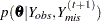. The two steps are iterated long enough for the results to reliably simulate an approximately independent draw of the missing values for a multiply imputed data set (Schafer 1997).

This creates a Markov chain , , ..., which converges in distribution to . Assuming the iterates converge to a stationary distribution, the goal is to simulate an approximately independent draw of the missing values from this distribution.

To validate the imputation results, you should repeat the process with different random number generators and starting values based on different initial parameter estimates.

The next three sections provide details for the imputation step, Bayesian estimation of the mean vector and covariance matrix, and the posterior step.

Imputation Step

In each iteration, starting with a given mean vector and covariance matrix , the imputation step draws values for the missing data from the conditional distribution given .

Suppose is the partitioned mean vector of two sets of variables, and , where is the mean vector for variables and is the mean vector for variables .

Also suppose

is the partitioned covariance matrix for these variables, where is the covariance matrix for variables , is the covariance matrix for variables , and is the covariance matrix between variables and variables .

By using the sweep operator (Goodnight 1979) on the pivots of the submatrix, the matrix becomes

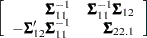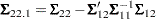
where 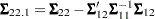can be used to compute the conditional covariance matrix of after controlling for .

For an observation with the preceding missing pattern, the conditional distribution of given is a multivariate normal distribution with the mean vector

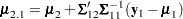and the conditional covariance matrix

Bayesian Estimation of the Mean Vector and Covariance Matrix

Suppose that 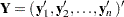is an matrix made up of independent vectors , each of which has a multivariate normal distribution with mean zero and covariance matrix . Then the SSCP matrix

has a Wishart distribution .

When each observation is distributed with a multivariate normal distribution with an unknown mean , then the CSSCP matrix

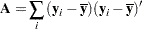has a Wishart distribution .

If has a Wishart distribution , then has an inverted Wishart distribution , where is the degrees of freedom and is the precision matrix (Anderson 1984).

Note that, instead of using the parameter for the inverted Wishart distribution, Schafer (1997) uses the parameter .

Suppose that each observation in the data matrix has a multivariate normal distribution with mean and covariance matrix . Then with a prior inverted Wishart distribution for and a prior normal distribution for

where is a fixed number.

The posterior distribution (Anderson 1984, p. 270; Schafer 1997, p. 152) is

where is the CSSCP matrix.

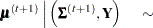
Posterior Step

In each iteration, the posterior step simulates the posterior population mean vector and covariance matrix from prior information for and , and the complete sample estimates.

You can specify the prior parameter information by using one of the following methods:

• PRIOR=JEFFREYS, which uses a noninformative prior

• PRIOR=INPUT=, which provides a prior information for in the data set. Optionally, it also provides a prior information for in the data set.

• PRIOR=RIDGE=, which uses a ridge prior

The next four subsections provide details of the posterior step for different prior distributions.

1. A Noninformative Prior

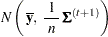
Without prior information about the mean and covariance estimates, you can use a noninformative prior by specifying the PRIOR=JEFFREYS option. The posterior distributions (Schafer 1997, p. 154) are

2. An Informative Prior for and

When prior information is available for the parameters and , you can provide it with a SAS data set that you specify with the PRIOR=INPUT= option:

To obtain the prior distribution for , PROC MI reads the matrix from observations in the data set with _TYPE_=‘COV’, and it reads from observations with _TYPE_=‘N’.

To obtain the prior distribution for , PROC MI reads the mean vector from observations with _TYPE_=‘MEAN’, and it reads from observations with _TYPE_=‘N_MEAN’. When there are no observations with _TYPE_=‘N_MEAN’, PROC MI reads from observations with _TYPE_=‘N’.

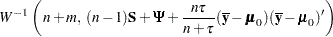
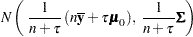
The resulting posterior distribution, as described in the section Bayesian Estimation of the Mean Vector and Covariance Matrix, is given by

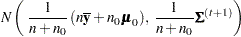where

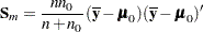3. An Informative Prior for

When the sample covariance matrix is singular or near singular, prior information about can also be used without prior information about to stabilize the inference about . You can provide it with a SAS data set that you specify with the PRIOR=INPUT= option.

To obtain the prior distribution for , PROC MI reads the matrix from observations in the data set with _TYPE_=‘COV’, and it reads from observations with _TYPE_=‘N’.

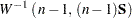
The resulting posterior distribution for (Schafer 1997, p. 156) is

Note that if the PRIOR=INPUT= data set also contains observations with _TYPE_=‘MEAN’, then a complete informative prior for both and will be used.

4. A Ridge Prior

A special case of the preceding adjustment is a ridge prior with = Diag (Schafer 1997, p. 156). That is, is a diagonal matrix with diagonal elements equal to the corresponding elements in .

You can request a ridge prior by using the PRIOR=RIDGE= option. You can explicitly specify the number in the PRIOR=RIDGE= option. Or you can implicitly specify the number by specifying the proportion in the PRIOR=RIDGE= option to request .

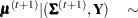
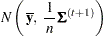
The posterior is then given by