The MI Procedure
- Overview
- Getting Started
-
Syntax

-
Details
Descriptive Statistics EM Algorithm for Data with Missing Values Statistical Assumptions for Multiple Imputation Missing Data Patterns Imputation Methods Monotone Methods for Data Sets with Monotone Missing Patterns Monotone and FCS Regression Methods Monotone and FCS Predictive Mean Matching Methods Monotone Propensity Score Method Monotone and FCS Discriminant Function Methods Monotone and FCS Logistic Regression Methods FCS Methods for Data Sets with Arbitrary Missing Patterns Checking Convergence in FCS Methods MCMC Method for Arbitrary Missing Multivariate Normal Data Producing Monotone Missingness with the MCMC Method MCMC Method Specifications Checking Convergence in MCMC Input Data Sets Output Data Sets Combining Inferences from Multiply Imputed Data Sets Multiple Imputation Efficiency Imputer’s Model Versus Analyst’s Model Parameter Simulation versus Multiple Imputation Summary of Issues in Multiple Imputation ODS Table Names ODS Graphics
-
Examples
EM Algorithm for MLE Monotone Propensity Score Method Monotone Regression Method Monotone Logistic Regression Method for CLASS Variables Monotone Discriminant Function Method for CLASS Variables FCS Method for Continuous Variables FCS Method for CLASS Variables FCS Method with Trace Plot MCMC Method Producing Monotone Missingness with MCMC Checking Convergence in MCMC Saving and Using Parameters for MCMC Transforming to Normality Multistage Imputation
- References
| Monotone and FCS Predictive Mean Matching Methods |
The predictive mean matching method is also an imputation method available for continuous variables. It is similar to the regression method except that for each missing value, it imputes a value randomly from a set of observed values whose predicted values are closest to the predicted value for the missing value from the simulated regression model (Heitjan and Little 1991; Schenker and Taylor 1996).
Following the description of the model in the section Monotone and FCS Regression Methods, the following steps are used to generate imputed values:
-
New parameters
 and
and  are drawn from the posterior predictive distribution of the parameters. That is, they are simulated from
  ,
,  , and
, and  . The variance is drawn as
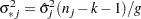
where
 is a
is a  random variate and
  is the number of nonmissing observations for
  . The regression coefficients are drawn as
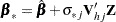
where
 is the upper triangular matrix in the Cholesky decomposition,
  , and
, and  is a vector of
  independent random normal variates.
 -
For each missing value, a predicted value

is computed with the covariate values
 .
. A set of
 observations whose corresponding predicted values are closest to
  is generated. You can specify with the K= option.
 The missing value is then replaced by a value drawn randomly from these
observed values.
The predictive mean matching method requires the number of closest observations to be specified. A smaller tends to increase the correlation among the multiple imputations for the missing observation and results in a higher variability of point estimators in repeated sampling. On the other hand, a larger tends to lessen the effect from the imputation model and results in biased estimators (Schenker and Taylor 1996, p. 430).
The predictive mean matching method ensures that imputed values are plausible; it might be more appropriate than the regression method if the normality assumption is violated (Horton and Lipsitz 2001, p. 246).