The LIFEREG Procedure
- Overview
-
Getting Started

-
Syntax
-
Details
Missing Values Model Specification Computational Method Supported Distributions Predicted Values Confidence Intervals Fit Statistics Probability Plotting INEST= Data Set OUTEST= Data Set XDATA= Data Set Computational Resources Bayesian Analysis Displayed Output for Classical Analysis Displayed Output for Bayesian Analysis ODS Table Names ODS Graphics
-
Examples
Motorette Failure Computing Predicted Values for a Tobit Model Overcoming Convergence Problems by Specifying Initial Values Analysis of Arbitrarily Censored Data with Interaction Effects Probability Plotting—Right Censoring Probability Plotting—Arbitrary Censoring Bayesian Analysis of Clinical Trial Data
- References
Example 50.7 Bayesian Analysis of Clinical Trial Data
Consider the data on melanoma patients from a clinical trial described in Ibrahim, Chen, and Sinha (2001). A partial listing of the data is shown in Output 50.7.1.
The survival time is modeled by a Weibull regression model with three covariates. An analysis of the right-censored survival data is performed with PROC LIFEREG to obtain Bayesian estimates of the regression coefficients by using the following SAS statements:
ods graphics on;
proc lifereg data=e1684;
   class Sex;
   model Survtime*Survcens(1)=Age Sex Perform / dist=Weibull;
   bayes WeibullShapePrior=gamma seed=9999;
run;
ods graphics off;
| Obs | survtime | survcens | age | sex | perform |
|---|---|---|---|---|---|
| 1 | 1.57808 | 2 | 35.9945 | 1 | 0 |
| 2 | 1.48219 | 2 | 41.9014 | 1 | 0 |
| 3 | 7.33425 | 1 | 70.2164 | 2 | 0 |
| 4 | 0.65479 | 2 | 58.1753 | 2 | 1 |
| 5 | 2.23288 | 2 | 33.7096 | 1 | 0 |
| 6 | 9.38356 | 1 | 47.9726 | 1 | 0 |
| 7 | 3.27671 | 2 | 31.8219 | 2 | 0 |
| 8 | 0.00000 | 1 | 72.3644 | 2 | 0 |
| 9 | 0.80274 | 2 | 40.7151 | 2 | 0 |
| 10 | 9.64384 | 1 | 32.9479 | 1 | 0 |
| 11 | 1.66575 | 2 | 35.9205 | 1 | 0 |
| 12 | 0.94247 | 2 | 40.5068 | 2 | 0 |
| 13 | 1.68767 | 2 | 57.0384 | 1 | 0 |
| 14 | 5.94247 | 2 | 63.1452 | 1 | 0 |
| 15 | 2.34247 | 2 | 62.0630 | 1 | 0 |
| 16 | 0.89863 | 2 | 56.5342 | 1 | 1 |
| 17 | 9.03288 | 1 | 22.9945 | 2 | 0 |
| 18 | 9.63014 | 1 | 18.4712 | 1 | 0 |
| 19 | 0.52603 | 2 | 41.2521 | 1 | 0 |
| 20 | 1.82192 | 2 | 29.5178 | 1 | 0 |
Maximum likelihood estimates of the model parameters shown in Output 50.7.2 are displayed by default.
| Analysis of Maximum Likelihood Parameter Estimates | ||||||
|---|---|---|---|---|---|---|
| Parameter | DF | Estimate | Standard Error | 95% Confidence Limits | ||
| Intercept | 1 | 2.4402 | 0.3716 | 1.7119 | 3.1685 | |
| age | 1 | -0.0115 | 0.0070 | -0.0253 | 0.0023 | |
| sex | 1 | 1 | -0.1170 | 0.1978 | -0.5046 | 0.2707 |
| sex | 2 | 0 | 0.0000 | . | . | . |
| perform | 1 | 0.2905 | 0.3222 | -0.3411 | 0.9220 | |
| Scale | 1 | 1.2537 | 0.0824 | 1.1021 | 1.4260 | |
| Weibull Shape | 1 | 0.7977 | 0.0524 | 0.7012 | 0.9073 | |
Since no prior distributions for the regression coefficients were specified, the default uniform improper distributions shown in the "Uniform Prior for Regression Coefficients" table in Output 50.7.3 are used. The specified gamma prior for the Weibull shape parameter is also shown in Output 50.7.3.
| Uniform Prior for Regression Coefficients |
|
|---|---|
| Parameter | Prior |
| Intercept | Constant |
| age | Constant |
| sex1 | Constant |
| perform | Constant |
| Independent Prior Distributions for Model Parameters | |||||
|---|---|---|---|---|---|
| Parameter | Prior Distribution | Hyperparameters | |||
| Weibull Shape | Gamma | Shape | 0.001 | Inverse Scale | 0.001 |
Fit statistics, descriptive statistics, interval statistics, and the sample parameter correlation matrix for the posterior sample are displayed in the tables in Output 50.7.4. Since noninformative prior distributions for the regression coefficients were used, the mean and standard deviations of the posterior distributions for the model parameters are close to the maximum likelihood estimates and standard errors.
| Fit Statistics | |
|---|---|
| DIC (smaller is better) | 875.251 |
| pD (effective number of parameters) | 4.984 |
| Posterior Summaries | ||||||
|---|---|---|---|---|---|---|
| Parameter | N | Mean | Standard Deviation |
Percentiles | ||
| 25% | 50% | 75% | ||||
| Intercept | 10000 | 2.4668 | 0.3862 | 2.1989 | 2.4621 | 2.7256 |
| age | 10000 | -0.0115 | 0.00733 | -0.0163 | -0.0115 | -0.00652 |
| sex1 | 10000 | -0.1255 | 0.2004 | -0.2584 | -0.1247 | 0.00817 |
| perform | 10000 | 0.3304 | 0.3317 | 0.1071 | 0.3188 | 0.5470 |
| WeibShape | 10000 | 0.7834 | 0.0518 | 0.7481 | 0.7815 | 0.8178 |
| Posterior Intervals | |||||
|---|---|---|---|---|---|
| Parameter | Alpha | Equal-Tail Interval | HPD Interval | ||
| Intercept | 0.050 | 1.7279 | 3.2368 | 1.7234 | 3.2264 |
| age | 0.050 | -0.0260 | 0.00263 | -0.0261 | 0.00244 |
| sex1 | 0.050 | -0.5197 | 0.2676 | -0.5260 | 0.2583 |
| perform | 0.050 | -0.2898 | 1.0072 | -0.3200 | 0.9726 |
| WeibShape | 0.050 | 0.6846 | 0.8905 | 0.6805 | 0.8849 |
| Posterior Correlation Matrix | |||||
|---|---|---|---|---|---|
| Parameter | Intercept | age | sex1 | perform | WeibShape |
| Intercept | 1.0000 | -.9018 | -.3099 | -.0888 | -.1140 |
| age | -.9018 | 1.0000 | -.0259 | -.0363 | 0.0493 |
| sex1 | -.3099 | -.0259 | 1.0000 | 0.1248 | 0.0371 |
| perform | -.0888 | -.0363 | 0.1248 | 1.0000 | -.0355 |
| WeibShape | -.1140 | 0.0493 | 0.0371 | -.0355 | 1.0000 |
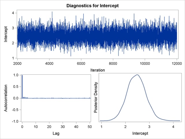
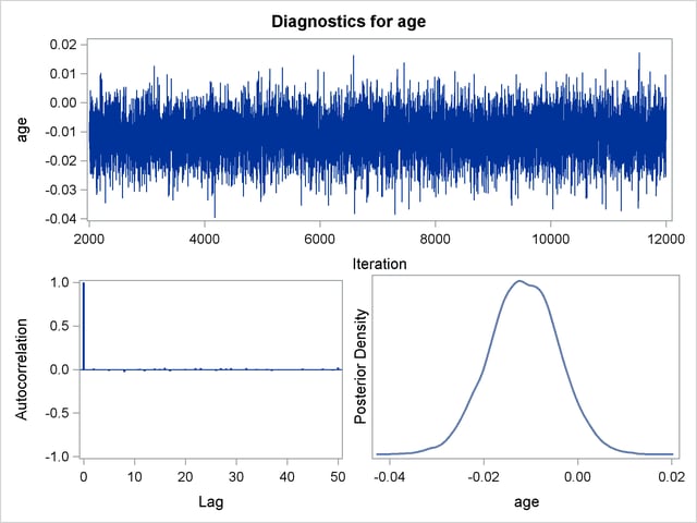
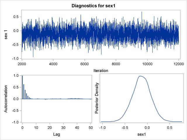
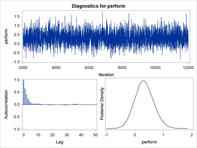
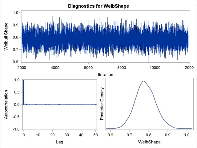
The default diagnostic statistics are displayed in Output 50.7.5. See the section Assessing Markov Chain Convergence for more details on Bayesian convergence diagnostics.
| Posterior Autocorrelations | ||||
|---|---|---|---|---|
| Parameter | Lag 1 | Lag 5 | Lag 10 | Lag 50 |
| Intercept | 0.0564 | 0.0030 | 0.0082 | 0.0234 |
| age | -0.0079 | -0.0184 | -0.0015 | 0.0239 |
| sex1 | 0.6293 | 0.0700 | 0.0055 | -0.0199 |
| perform | 0.6514 | 0.0773 | 0.0397 | -0.0123 |
| WeibShape | 0.0719 | -0.0083 | -0.0062 | 0.0112 |
| Geweke Diagnostics | ||
|---|---|---|
| Parameter | z | Pr > |z| |
| Intercept | 0.4962 | 0.6198 |
| age | -0.4119 | 0.6804 |
| sex1 | -0.2519 | 0.8011 |
| perform | -0.1049 | 0.9165 |
| WeibShape | -0.6573 | 0.5110 |
| Effective Sample Sizes | |||
|---|---|---|---|
| Parameter | ESS | Autocorrelation Time |
Efficiency |
| Intercept | 7476.1 | 1.3376 | 0.7476 |
| age | 10000.0 | 1.0000 | 1.0000 |
| sex1 | 2482.1 | 4.0288 | 0.2482 |
| perform | 2174.0 | 4.5998 | 0.2174 |
| WeibShape | 8538.8 | 1.1711 | 0.8539 |
Trace, autocorrelation, and density plots for the seven model parameters are shown in Output 50.7.6 through Output 50.7.10. These plots show no indication that the Markov chains have not converged. See the sections Assessing Markov Chain Convergence and Visual Analysis via Trace Plots for more information about assessing the convergence of the chain of posterior samples.