The LIFEREG Procedure
- Overview
-
Getting Started

-
Syntax
-
Details
Missing Values Model Specification Computational Method Supported Distributions Predicted Values Confidence Intervals Fit Statistics Probability Plotting INEST= Data Set OUTEST= Data Set XDATA= Data Set Computational Resources Bayesian Analysis Displayed Output for Classical Analysis Displayed Output for Bayesian Analysis ODS Table Names ODS Graphics
-
Examples
Motorette Failure Computing Predicted Values for a Tobit Model Overcoming Convergence Problems by Specifying Initial Values Analysis of Arbitrarily Censored Data with Interaction Effects Probability Plotting—Right Censoring Probability Plotting—Arbitrary Censoring Bayesian Analysis of Clinical Trial Data
- References
Example 50.4 Analysis of Arbitrarily Censored Data with Interaction Effects
The artificial data in this example are from a study of the natural recovery time of mice after injection of a certain toxin. Twenty mice were grouped by sex (sex: 1 = Male, 2 = Female) with equal sizes. Their ages (in days) were recorded at the injection. Their recovery times (in minutes) were also recorded. Toxin density in blood was used to decide whether a mouse recovered. Mice were checked at two times for recovery. If a mouse had recovered at the first time, the observation is left censored, and no further measurement is made. The variable time1 is set to missing and time2 is set to the measurement time to indicate left censoring. If a mouse had not recovered at the first time, it was checked later at a second time. If it had recovered by the second measurement time, the observation is interval censored, and the variable time1 is set to the first measurement time and time2 is set to the second measurement time. If there was no recovery at the second measurement, the observation is right censored, and time1 is set to the second measurement time and time2 is set to missing to indicate right censoring.
The following statements create a SAS data set containing the data from the experiment:
title 'Natural Recovery Time';
data mice;
   input sex age time1 time2 ;
   datalines;
1  57  631   631
1  45  .     170
1  54  227   227
1  43  143   143
1  64  916   .
1  67  691   705
1  44  100   100
1  59  730   .
1  47  365   365
1  74  1916  1916
2  79  1326  .
2  75  837   837
2  84  1200  1235
2  54  .     365
2  74  1255  1255
2  71  1823  .
2  65  537   637
2  33  583   683
2  77  955   .
2  46  577   577
;
The following SAS statements create the SAS data sets xrow1 and xrow2:
data xrow1;
   input sex age time1 time2 ;
   datalines;
1  50  .  .
;

data xrow2;
   input sex age time1 time2 ;
   datalines;
2  60.6  .  .
;
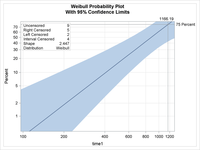
The following SAS statements fit a Weibull model with age, sex, and an age-by-sex interaction term as covariates, and create a plot of predicted probabilities against recovery time for the fixed values of age and sex specified in the SAS data set xrow1:
ods graphics on;
proc lifereg data=mice xdata=xrow1;
   class sex  ;
   model (time1, time2) = age sex age*sex / dist=Weibull;

   probplot  / nodata
       plower=.5
       vref(intersect) = 75
       vreflab = '75 Percent'
       ;
   inset;
run;
Standard output is shown in Output 50.4.1. Tables containing general model information, Type III tests for the main effects and interaction terms, and parameter estimates are created.
| Natural Recovery Time |
| Model Information | |
|---|---|
| Data Set | WORK.MICE |
| Dependent Variable | Log(time1) |
| Dependent Variable | Log(time2) |
| Number of Observations | 20 |
| Noncensored Values | 9 |
| Right Censored Values | 5 |
| Left Censored Values | 2 |
| Interval Censored Values | 4 |
| Number of Parameters | 5 |
| Name of Distribution | Weibull |
| Log Likelihood | -25.91033295 |
| Type III Analysis of Effects | |||
|---|---|---|---|
| Effect | DF | Wald Chi-Square |
Pr > ChiSq |
| age | 1 | 33.8496 | <.0001 |
| sex | 1 | 14.0245 | 0.0002 |
| age*sex | 1 | 10.7196 | 0.0011 |
| Analysis of Maximum Likelihood Parameter Estimates | ||||||||
|---|---|---|---|---|---|---|---|---|
| Parameter | DF | Estimate | Standard Error | 95% Confidence Limits | Chi-Square | Pr > ChiSq | ||
| Intercept | 1 | 5.4110 | 0.5549 | 4.3234 | 6.4986 | 95.08 | <.0001 | |
| age | 1 | 0.0250 | 0.0086 | 0.0081 | 0.0419 | 8.42 | 0.0037 | |
| sex | 1 | 1 | -3.9808 | 1.0630 | -6.0643 | -1.8974 | 14.02 | 0.0002 |
| sex | 2 | 0 | 0.0000 | . | . | . | . | . |
| age*sex | 1 | 1 | 0.0613 | 0.0187 | 0.0246 | 0.0980 | 10.72 | 0.0011 |
| age*sex | 2 | 0 | 0.0000 | . | . | . | . | . |
| Scale | 1 | 0.4087 | 0.0900 | 0.2654 | 0.6294 | |||
| Weibull Shape | 1 | 2.4468 | 0.5391 | 1.5887 | 3.7682 | |||
The following two plots display the predicted probability against the recovery time for two different populations. Output 50.4.2 is created with the PROBPLOT statement with the option XDATA= xrow1, which specifies the population with sex = 1, age = 50. Output 50.4.3 is created with the PROBPLOT statement with the option XDATA= xrow2, which specifies the population with sex = 2, age = 60.6. These are the default values that the LIFEREG procedure would use for the probability plot if the XDATA= option had not been specified. Reference lines are used to display specified predicted probability points and their relative locations in the plot.
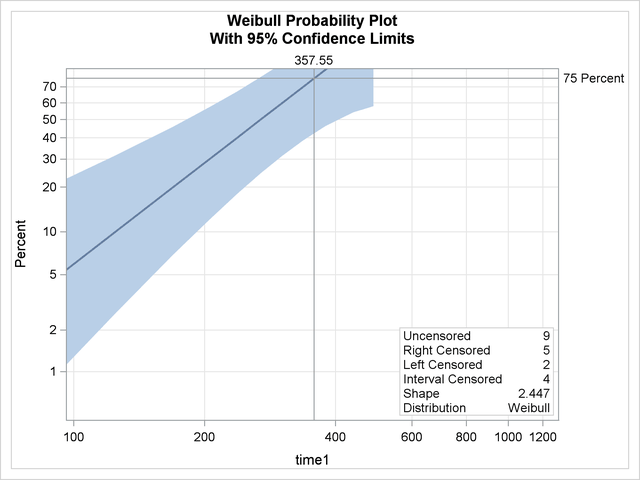
The following SAS statements fit a Weibull model with age, sex, and an age-by-sex interaction term as covariates, and create the plot of predicted probabilities against recovery time shown in Output 50.4.3, for the fixed values of age and sex specified in the SAS data set xrow2:
proc lifereg data=mice xdata=xrow2;
   class sex  ;
   model (time1, time2) = age sex age*sex / dist=Weibull;

   probplot  / nodata
       plower=.5
       vref(intersect) = 75
       vreflab = '75 Percent'
       ;
   inset;
run;
title;
ods graphics off;