The LIFEREG Procedure
- Overview
-
Getting Started

-
Syntax
-
Details
Missing Values Model Specification Computational Method Supported Distributions Predicted Values Confidence Intervals Fit Statistics Probability Plotting INEST= Data Set OUTEST= Data Set XDATA= Data Set Computational Resources Bayesian Analysis Displayed Output for Classical Analysis Displayed Output for Bayesian Analysis ODS Table Names ODS Graphics
-
Examples
Motorette Failure Computing Predicted Values for a Tobit Model Overcoming Convergence Problems by Specifying Initial Values Analysis of Arbitrarily Censored Data with Interaction Effects Probability Plotting—Right Censoring Probability Plotting—Arbitrary Censoring Bayesian Analysis of Clinical Trial Data
- References
| Modeling Right-Censored Failure Time Data |
The following example demonstrates how you can use the LIFEREG procedure to fit a model to right-censored failure time data.
Suppose you conduct a study of two headache pain relievers. You divide patients into two groups, with each group receiving a different type of pain reliever. You record the time taken (in minutes) for each patient to report headache relief. Because some of the patients never report relief for the entire study, some of the observations are censored.
The following DATA step creates the SAS data set headache:
data Headache;
   input Minutes Group Censor @@;
   datalines;
11  1  0   12  1  0   19  1  0   19  1  0
19  1  0   19  1  0   21  1  0   20  1  0
21  1  0   21  1  0   20  1  0   21  1  0
20  1  0   21  1  0   25  1  0   27  1  0
30  1  0   21  1  1   24  1  1   14  2  0
16  2  0   16  2  0   21  2  0   21  2  0
23  2  0   23  2  0   23  2  0   23  2  0
25  2  1   23  2  0   24  2  0   24  2  0
26  2  1   32  2  1   30  2  1   30  2  0
32  2  1   20  2  1
;
The data set Headache contains the variable Minutes, which represents the reported time to headache relief; the variable Group, the group to which the patient is assigned; and the variable Censor, a binary variable indicating whether the observation is censored. Valid values of the variable Censor are 0 (no) and 1 (yes). Figure 50.1 shows the first five records of the data set Headache.
| Obs | Minutes | Group | Censor |
|---|---|---|---|
| 1 | 11 | 1 | 0 |
| 2 | 12 | 1 | 0 |
| 3 | 19 | 1 | 0 |
| 4 | 19 | 1 | 0 |
| 5 | 19 | 1 | 0 |
The following statements invoke the LIFEREG procedure:
proc lifereg data=Headache;
   class Group;
   model Minutes*Censor(1)=Group;
   output out=New cdf=Prob;
run;
The CLASS statement specifies the variable Group as the classification variable. The MODEL statement syntax indicates that the response variable Minutes is right censored when the variable Censor takes the value 1. The MODEL statement specifies the variable Group as the single explanatory variable. Because the MODEL statement does not specify the DISTRIBUTION= option, the LIFEREG procedure fits the default type 1 extreme-value distribution by using  as the response. This is equivalent to fitting the Weibull distribution.
The OUTPUT statement creates the output data set New. In addition to containing the variables in the original data set Headache, the SAS data set New also contains the variable Prob. This new variable is created by the CDF= option to contain the estimates of the cumulative distribution function evaluated at the observed response.
The results of this analysis are displayed in the following figures.
| Model Information | |
|---|---|
| Data Set | WORK.HEADACHE |
| Dependent Variable | Log(Minutes) |
| Censoring Variable | Censor |
| Censoring Value(s) | 1 |
| Number of Observations | 38 |
| Noncensored Values | 30 |
| Right Censored Values | 8 |
| Left Censored Values | 0 |
| Interval Censored Values | 0 |
| Number of Parameters | 3 |
| Name of Distribution | Weibull |
| Log Likelihood | -9.37930239 |
| Class Level Information | ||
|---|---|---|
| Name | Levels | Values |
| Group | 2 | 1 2 |
Figure 50.2 displays the class level information and model fitting information. There are 30 uncensored observations and 8 right-censored observations. The log likelihood for the Weibull distribution is –9.3793. The log-likelihood value can be used to compare the goodness of fit for nested models with different covariates, but with the same distribution.
| Fit Statistics | |
|---|---|
| -2 Log Likelihood | 18.759 |
| AIC (smaller is better) | 24.759 |
| AICC (smaller is better) | 25.464 |
| BIC (smaller is better) | 29.671 |
| Fit Statistics (Unlogged Response) | |
|---|---|
| -2 Log Likelihood | 199.747 |
| Weibull AIC (smaller is better) | 205.747 |
| Weibull AICC (smaller is better) | 206.453 |
| Weibull BIC (smaller is better) | 210.660 |
Figure 50.3 displays fit statistics for the model. The "Fit Statistics" table displays statistics based on the maximum extreme-value log likelihood fit by using as the response. These statistics are useful in comparing the fit of a different model when the fit criteria from the model that you compare is also based on the log likelihood using as the response. The "Fit Statistics (Unlogged Response)" table is based on the maximum Weibull log likelihood using Minutes as the response. The AIC, BIC, and AICC statistics in this table can be used to compare models with different covariates, in addition to models with different distributions, as long as the fit statistics for the models that you compare use Minutes as the response.
| Analysis of Maximum Likelihood Parameter Estimates | ||||||||
|---|---|---|---|---|---|---|---|---|
| Parameter | DF | Estimate | Standard Error | 95% Confidence Limits | Chi-Square | Pr > ChiSq | ||
| Intercept | 1 | 3.3091 | 0.0589 | 3.1938 | 3.4245 | 3161.70 | <.0001 | |
| Group | 1 | 1 | -0.1933 | 0.0786 | -0.3473 | -0.0393 | 6.05 | 0.0139 |
| Group | 2 | 0 | 0.0000 | . | . | . | . | . |
| Scale | 1 | 0.2122 | 0.0304 | 0.1603 | 0.2809 | |||
| Weibull Shape | 1 | 4.7128 | 0.6742 | 3.5604 | 6.2381 | |||
The table of parameter estimates is displayed in Figure 50.4. Both the intercept and the slope parameter for the variable group are significantly different from 0 at the 0.05 level. Because the variable group has only one degree of freedom, parameter estimates are given for only one level of the variable group (group=1). However, the estimate for the intercept parameter provides a baseline for group=2.
The resulting model is as follows:
 |
Note that the Weibull shape parameter for this model is the reciprocal of the extreme-value scale parameter estimate shown in Figure 50.4 ( ).
).
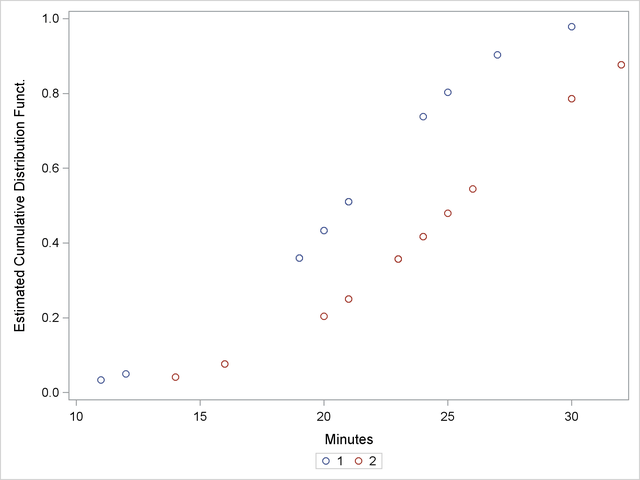
The following statements produce a graph of the cumulative distribution values versus the variable Minutes.
proc sgplot data=New;
   scatter x=Minutes y=Prob / group=Group;
   discretelegend;
run;
Figure 50.5 displays the estimated cumulative distribution function values contained in the output data set New for each group.