The LIFEREG Procedure

By default, the LIFEREG procedure computes initial values for the parameters by using ordinary least squares (OLS) and ignoring censoring. This might not be the best set of starting values for a given set of data. For example, if there are extreme values in your data, the OLS fit might be excessively influenced by the extreme observations, causing an overflow or convergence problems. See Example 50.3 for one way to deal with convergence problems.

You can specify the INITIAL= option in the MODEL statement to override these starting values. You can also specify the INTERCEPT=, SCALE=, and SHAPE= options to set initial values of the intercept, scale, and shape parameters. For models with multilevel interaction effects, it is a little difficult to use the INITIAL= option to provide starting values for all parameters. In this case, you can use the INEST= data set. See the section INEST= Data Set for details. The INEST= data set overrides all previous specifications for starting values of parameters.

The rank of the design matrix is estimated before the model is fit. Columns of that are judged linearly dependent on other columns have the corresponding parameters set to zero. The test for linear dependence is controlled by the SINGULAR= option in the MODEL statement. Variables are included in the model in the order in which they are listed in the MODEL statement with the continuous variables included in the model before any classification variables.

The log-likelihood function is maximized by means of a ridge-stabilized Newton-Raphson algorithm. The maximized value of the log likelihood can take positive or negative values, depending on the specified model and the values of the maximum likelihood estimates of the model parameters.

If convergence of the maximum likelihood estimates is attained, a Type III chi-square test statistic is computed for each effect, testing whether there is any contribution from any of the levels of the effect. This statistic is computed as a quadratic form in the appropriate parameter estimates by using the corresponding submatrix of the asymptotic covariance matrix estimate. See Chapter 41, The GLM Procedure, and Chapter 15, The Four Types of Estimable Functions, for more information about Type III estimable functions. The asymptotic covariance matrix is computed as the inverse of the observed information matrix. Note that if the NOINT option is specified and CLASS variables are used, the first CLASS variable contains a contribution from an intercept term. The results are displayed in an ODS table named "Type3Analysis." Chi-square tests for individual parameters are Wald tests based on the observed information matrix and the parameter estimates. If an effect has a single degree of freedom in the parameter estimates table, the chi-square test for this parameter is equivalent to the Type III test for this effect.

Before SAS 8.2, a multiple-degree-of-freedom statistic was computed for each effect to test for contribution from any level of the effect. In general, the Type III test statistic in a main-effect-only model (no interaction terms) will be equal to the previously computed effect statistic, unless there are collinearities among the effects. If there are collinearities, the Type III statistic will adjust for them, and the value of the Type III statistic and the number of degrees of freedom might not be equal to those of the previous effect statistic.

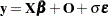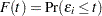
Suppose there are observations from the model (or if there is an offset variable), where is an matrix of covariate values (including the intercept), is a vector of responses, is a vector of offset variable values, and is a vector of errors with survival function , cumulative distribution function , and probability density function . That is, 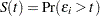, , and , where is a component of the error vector. Then, if all the responses are observed, the log likelihood, , can be written as

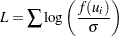where .

If some of the responses are left, right, or interval censored, the log likelihood can be written as

with the first sum over uncensored observations, the second sum over right-censored observations, the third sum over left-censored observations, the last sum over interval-censored observations, and

where is the lower end of a censoring interval.

If the response is specified in the binomial format, events/trials, then the log-likelihood function is

where is the number of events and is the number of trials for the th observation. In this case, . For the symmetric distributions, logistic and normal, this is the same as . Additional information about censored and limited dependent variable models can be found in Kalbfleisch and Prentice (1980) and Maddala (1983).

The estimated covariance matrix of the parameter estimates is computed as the negative inverse of , which is the information matrix of second derivatives of with respect to the parameters evaluated at the final parameter estimates. If is not positive definite, a positive-definite submatrix of is inverted, and the remaining rows and columns of the inverse are set to zero. If some of the parameters, such as the scale and intercept, are restricted, the corresponding elements of the estimated covariance matrix are set to zero. The standard error estimates for the parameter estimates are taken as the square roots of the corresponding diagonal elements.

For restrictions placed on the intercept, scale, and shape parameters, one-degree-of-freedom Lagrange multiplier test statistics are computed. These statistics are computed as

where is the derivative of the log likelihood with respect to the restricted parameter at the restricted maximum and

where the 1 subscripts refer to the restricted parameter and the 2 subscripts refer to the unrestricted parameters. The information matrix is evaluated at the restricted maximum. These statistics are asymptotically distributed as chi-squares with one degree of freedom under the null hypothesis that the restrictions are valid, provided that some regularity conditions are satisfied. Refer to Rao (1973, p. 418) for a more complete discussion. It is possible for these statistics to be missing if the observed information matrix is not positive definite. Higher-degree-of-freedom tests for multiple restrictions are not currently computed.

A Lagrange multiplier test statistic is computed to test this constraint. Notice that this test statistic is comparable to the Wald test statistic for testing that the scale is one. The Wald statistic is the result of squaring the difference of the estimate of the scale parameter from one and dividing this by the square of its estimated standard error.