The ENTROPY Procedure (Experimental)
- Overview
-
Getting Started

-
Syntax
-
DetailsGeneralized Maximum EntropyGeneralized Cross EntropyMoment Generalized Maximum EntropyMaximum Entropy-Based Seemingly Unrelated RegressionGeneralized Maximum Entropy for Multinomial Discrete Choice ModelsCensored or Truncated Dependent VariablesInformation MeasuresParameter Covariance For GCEParameter Covariance For GCE-MStatistical TestsMissing ValuesInput Data SetsOutput Data SetsODS Table NamesODS Graphics
-
Examples
- References
You can use prior information about the parameters or the residuals to improve the efficiency of the estimates. Some authors prefer the terms pre-sample or pre-data over the term prior when used with maximum entropy to avoid confusion with Bayesian methods. The maximum entropy method described here does not use Bayes’ rule when including prior information in the estimation.
To perform regression, the ENTROPY procedure uses a generalization of maximum entropy called generalized maximum entropy. In maximum entropy estimation, the unknowns are probabilities. Generalized maximum entropy expands the set of problems that
can be solved by introducing the concept of support points. Generalized maximum entropy still estimates probabilities, but these are the probabilities of a support point. Support points
are used to map the ![]() domain of the maximum entropy to the any finite range of values.
domain of the maximum entropy to the any finite range of values.
Prior information, such as expected ranges for the parameters or the residuals, is added by specifying support points for the parameters or the residuals. Support points are points in one dimension that specify the expected domain of the parameter or the residual. The wider the domain specified, the less efficient your parameter estimates are (the more variance they have). Specifying more support points in the same width interval also improves the efficiency of the parameter estimates at the cost of more computation. Golan, Judge, and Miller (1996) show that the gains in efficiency fall off for adding more than five support points. You can specify between 2 to 256 support points in the ENTROPY procedure.
If you have only a small amount of data, the estimates are very sensitive to your selection of support points and weights. For larger data sets, incorrect priors are discounted if they are not supported by the data.
Consider the data set generated by the following SAS statements:
data prior;
   do by = 1 to 100;
      do t = 1 to 10;
         y = 2*t + 5 * rannor(4);
         output;
      end;
   end;
run;
The PRIOR data set contains 100 samples of 10 observations each from the population
You can estimate these samples using PROC ENTROPY as
proc entropy data=prior outest=parm1 noprint;
   model y = t ;
   by by;
run;
The 100 estimates are summarized by using the following SAS statements:
proc univariate data=parm1;
   var t;
run;
The summary statistics from PROC UNIVARIATE are shown in Figure 13.11. The true value of the coefficient T is 2.0, demonstrating that maximum entropy estimates tend to be biased.
Now assume that you have prior information about the slope and the intercept for this model. You are reasonably confident that the slope is 2 and you are less confident that intercept is zero. To specify prior information about the parameters, use the PRIORS statement.
There are two parts to the prior information specified in the PRIORS statement. The first part is the support points for a
parameter. The support points specify the domain of the parameter. For example, the following statement sets the support points
-1000 and 1000 for the parameter associated with variable T:
priors t -1000 1000;
This means that the coefficient lies in the interval ![]() . If the estimated value of the coefficient is actually outside of this interval, the estimation will not converge. In the
previous PRIORS statement, no weights were specified for the support points, so uniform weights are assumed. This implies
that the coefficient has a uniform probability of being in the interval
. If the estimated value of the coefficient is actually outside of this interval, the estimation will not converge. In the
previous PRIORS statement, no weights were specified for the support points, so uniform weights are assumed. This implies
that the coefficient has a uniform probability of being in the interval ![]() .
.
The second part of the prior information is the weights on the support points. For example, the following statements sets
the support points 10, 15, 20, and 25 with weights 1, 5, 5, and 1 respectively for the coefficient of T:
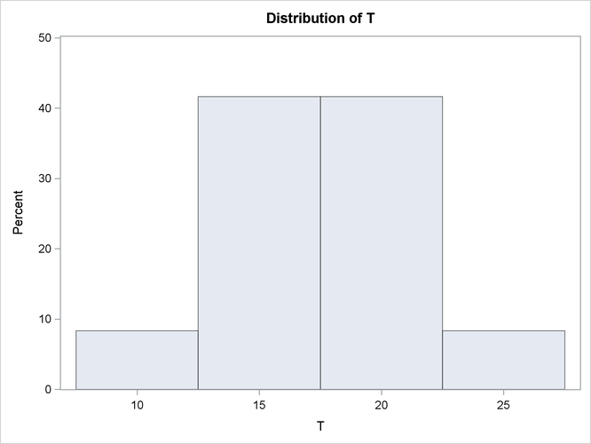
priors t 10(1) 15(5) 20(5) 25(1);
This creates the prior distribution on the coefficient shown in Figure 13.12. The weights are automatically normalized so that they sum to one.
For the PRIOR data set created previously, the expected value of the coefficient of T is 2. The following SAS statements reestimate the parameters with a prior weight specified for each one.
proc entropy data=prior outest=parm2 noprint;
   priors t 0(1) 2(3) 4(1)
          intercept -100(.5) -10(1.5) 0(2) 10(1.5) 100(0.5);
   model y = t;
   by by;
run;
The priors on the coefficient of T express a confident view of the value of the coefficient. The priors on INTERCEPT express a more diffuse view on the value
of the intercept. The following PROC UNIVARIATE statement computes summary statistics from the estimations:
proc univariate data=parm2;
   var t;
run;
The summary statistics for the distribution of the estimates of T are shown in Figure 13.13.
The prior information improves the estimation of the coefficient of T dramatically. The downside of specifying priors comes when they are incorrect. For example, say the priors for this model
were specified as
priors t -2(1) 0(3) 2(1);
to indicate a prior centered on zero instead of two.
The resulting summary statistics shown in Figure 13.14 indicate how the estimation is biased away from the solution.
The more data available for estimation, the less sensitive the parameters are to the priors. If the number of observations in each sample is 50 instead of 10, then the summary statistics shown in Figure 13.15 are produced. The prior information is not supported by the data, so it is discounted.