The ENTROPY Procedure (Experimental)
- Overview
-
Getting Started

-
Syntax
-
DetailsGeneralized Maximum EntropyGeneralized Cross EntropyMoment Generalized Maximum EntropyMaximum Entropy-Based Seemingly Unrelated RegressionGeneralized Maximum Entropy for Multinomial Discrete Choice ModelsCensored or Truncated Dependent VariablesInformation MeasuresParameter Covariance For GCEParameter Covariance For GCE-MStatistical TestsMissing ValuesInput Data SetsOutput Data SetsODS Table NamesODS Graphics
-
Examples
- References
In practice, you might find that variables are not always measured throughout their natural ranges. A given variable might be recorded continuously in a range, but, outside of that range, only the endpoint is denoted. In other words, say that the data generating process is:
However, you observe the following:
![\[ y^{\star }_\mi {i} = \left\{ \begin{array}{r@{\quad :\quad }l} ub & y_\mi {i} \ge ub \\ \mb{x}_\mi {i} \mb{\beta } + \epsilon & lb < y_\mi {i} < ub \\ lb & y_\mi {i} \le \mi{lb} \end{array} \right. \]](images/etsug_entropy0109.png)
The primal problem is simply a slight modification of the primal formulation for GME-GCE. You specify different supports for
the errors in the truncated or censored region, perhaps reflecting some nonsample information. Then the data constraints are
modified. The constraints that arise in the censored areas are changed to inequality constraints (Golan, Judge, and Perloff,
1997). Let the variable ![]() denote the observations of the explanatory variable where censoring occurs from the top,
denote the observations of the explanatory variable where censoring occurs from the top, ![]() from the bottom, and
from the bottom, and ![]() in the middle region (no censoring). Let,
in the middle region (no censoring). Let, ![]() be the supports for the observations at the upper bound,
be the supports for the observations at the upper bound, ![]() lower bound, and
lower bound, and ![]() in the middle.
in the middle.
You have:
![\[ \left[ \begin{array}{c} \mb{y} ^\mi {u} \ge \mi{ub} \\ \mb{y} ^\mi {a} \\ \mb{y} ^\mi {l} \le \mi{lb} \end{array} \right] = \left[ \begin{array}{c} \mb{X}^{u} \\ \mb{X}^{a} \\ \mb{X}^{l} \end{array} \right] \mb{Z} \mb{p} + \left[ \begin{array}{c} \mb{V}^{u}\mb{w} ^{u} \\ \mb{V}^{a}\mb{w} ^{a} \\ \mb{V}^{l}\mb{w} ^{l} \end{array} \right] \]](images/etsug_entropy0116.png)
The primal problem then becomes
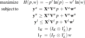
PROC ENTROPY requires that the number of supports be identical for all three regions.
Alternatively, you can think of cases where the dependent variable is observed continuously for most of its range. However, the variable’s range is reported for some observations. Such data is often found in highly disaggregated state level employment measures.
![\[ y^{\star }_\mi {i} = \left\{ \begin{array}{r@{\quad :\quad }l} \emph{missing} & l_1 \le y \le r_1 \\ \vdots & \vdots \\ \emph{missing} & l_\mi {k} \le y \le r_\mi {k} \\ \mb{x} _\mi {i} \mb{\beta } + \epsilon & otherwise \\ \end{array} \right. \]](images/etsug_entropy0118.png)
Just as in the censored case, each range yields two inequality constraints for each observation in that range.