The ENTROPY Procedure (Experimental)
- Overview
-
Getting Started

-
Syntax

-
Details
 Generalized Maximum EntropyGeneralized Cross EntropyMoment Generalized Maximum EntropyMaximum Entropy-Based Seemingly Unrelated RegressionGeneralized Maximum Entropy for Multinomial Discrete Choice ModelsCensored or Truncated Dependent VariablesInformation MeasuresParameter Covariance For GCEParameter Covariance For GCE-MStatistical TestsMissing ValuesInput Data SetsOutput Data SetsODS Table NamesODS Graphics
 -
Examples

- References
Factorial experiments are useful for studying the effects of various factors on a response. For the practitioner constrained to the use of OLS regression, there must be replication to estimate all of the possible main and interaction effects in a factorial experiment. Using OLS regression to analyze unreplicated experimental data results in zero degrees of freedom for error in the ANOVA table, since there are as many parameters as observations. This situation leaves the experimenter unable to compute confidence intervals or perform hypothesis testing on the parameter estimates.
Several options are available when replication is impossible. The higher-order interactions can be assumed to have negligible effects, and their degrees of freedom can be pooled to create the error degrees of freedom used to perform inference on the lower-order estimates. Or, if a preliminary experiment is being run, a normal probability plot of all effects can provide insight as to which effects are significant, and therefore focused, in a later, more complete experiment.
The following example illustrates the probability plot methodology and the alternative by using PROC ENTROPY. Consider a ![]() factorial model with no replication. The data are taken from Myers and Montgomery (1995).
factorial model with no replication. The data are taken from Myers and Montgomery (1995).
data rate;
   do a=-1,1; do b=-1,1; do c=-1,1; do d=-1,1;
      input y @@;
      ab=a*b; ac=a*c; ad=a*d; bc=b*c; bd=b*d; cd=c*d;
      abc=a*b*c; abd=a*b*d; acd=a*c*d; bcd=b*c*d;
      abcd=a*b*c*d;
      output;
   end; end; end; end;
   datalines;
   45 71 48 65 68 60 80 65 43 100 45 104 75 86 70 96
   ;
run;
Analyze the data by using PROC REG, then output the resulting estimates.
proc reg data=rate outest=regout;
   model y=a b c d ab ac ad bc bd cd abc abd acd bcd abcd;
run;

proc transpose data=regout out=ploteff name=effect prefix=est;
   var a b c d ab ac ad bc bd cd abc abd acd bcd abcd;
run;
Now the normal scores for the estimates can be computed with the rank procedure as follows:
proc rank data=ploteff normal=blom out=qqplot;
   var est1;
   ranks normalq;
run;
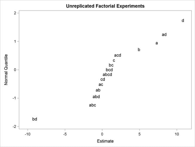
To create the probability plot, simply plot the estimates versus their normal scores by using PROC SGPLOT as follows:
title "Unreplicated Factorial Experiments";
proc sgplot data=qqplot;
   scatter x=est1 y=normalq / markerchar=effect
                              markercharattrs=(size=10pt);
   xaxis label="Estimate";
   yaxis label="Normal Quantile";
run;
The plot shown in Output 13.2.1 displays evidence that the a, b, d, ad, and bd estimates do not fit into the purely random normal model, which suggests that they may have some significant effect on the
response variable. To verify this, fit a reduced model that contains only these effects.
proc reg data=rate;
   model y=a b d ad bd;
run;
The estimates for the reduced model are shown in Output 13.2.2.
Output 13.2.2: Reduced Model OLS Estimates
| Unreplicated Factorial Experiments |
| Parameter Estimates | |||||
|---|---|---|---|---|---|
| Variable | DF | Parameter Estimate |
Standard Error |
t Value | Pr > |t| |
| Intercept | 1 | 70.06250 | 1.10432 | 63.44 | <.0001 |
| a | 1 | 7.31250 | 1.10432 | 6.62 | <.0001 |
| b | 1 | 4.93750 | 1.10432 | 4.47 | 0.0012 |
| d | 1 | 10.81250 | 1.10432 | 9.79 | <.0001 |
| ad | 1 | 8.31250 | 1.10432 | 7.53 | <.0001 |
| bd | 1 | -9.06250 | 1.10432 | -8.21 | <.0001 |
These results support the probability plot methodology.
PROC ENTROPY can directly estimate the full model without having to rely upon the probability plot for insight into which effects can be significant. To illustrate this, PROC ENTROPY is run by using default parameter and error supports in the following statements:
proc entropy data=rate;
   model y=a b c d ab ac ad bc bd cd abc abd acd bcd abcd;
run;
The resulting GME estimates are shown in Output 13.2.3. Note that the parameter estimates associated with the a, b, d, ad, and bd effects are all significant.
Output 13.2.3: Full Model Entropy Results
| Unreplicated Factorial Experiments |
| GME Variable Estimates | ||||
|---|---|---|---|---|
| Variable | Estimate | Approx Std Err | t Value | Approx Pr > |t| |
| a | 5.688414 | 0.7911 | 7.19 | <.0001 |
| b | 2.988032 | 0.5464 | 5.47 | <.0001 |
| c | 0.234331 | 0.1379 | 1.70 | 0.1086 |
| d | 9.627308 | 0.9765 | 9.86 | <.0001 |
| ab | -0.01386 | 0.0270 | -0.51 | 0.6149 |
| ac | -0.00054 | 0.00325 | -0.16 | 0.8712 |
| ad | 6.833076 | 0.8627 | 7.92 | <.0001 |
| bc | 0.113908 | 0.0941 | 1.21 | 0.2435 |
| bd | -7.68105 | 0.9053 | -8.48 | <.0001 |
| cd | 0.00002 | 0.000364 | 0.05 | 0.9569 |
| abc | -0.14876 | 0.1087 | -1.37 | 0.1900 |
| abd | -0.0399 | 0.0516 | -0.77 | 0.4509 |
| acd | 0.466938 | 0.1961 | 2.38 | 0.0300 |
| bcd | 0.059581 | 0.0654 | 0.91 | 0.3756 |
| abcd | 0.024785 | 0.0387 | 0.64 | 0.5312 |
| Intercept | 69.87294 | 1.1403 | 61.28 | <.0001 |
