The HPSEVERITY Procedure
- Overview
-
Getting Started

-
Syntax
-
DetailsPredefined DistributionsCensoring and TruncationParameter Estimation MethodDetails of Optimization AlgorithmsParameter InitializationEstimating Regression EffectsEmpirical Distribution Function Estimation MethodsStatistics of FitDistributed and Multithreaded ComputationDefining a Severity Distribution Model with the FCMP ProcedurePredefined Utility FunctionsCustom Objective FunctionsInput Data SetsOutput Data SetsDisplayed Output
-
ExamplesDefining a Model for Gaussian DistributionDefining a Model for the Gaussian Distribution with a Scale ParameterDefining a Model for Mixed-Tail DistributionsFitting a Scaled Tweedie Model with RegressorsFitting Distributions to Interval-Censored DataBenefits of Distributed and Multithreaded ComputingEstimating Parameters Using Cramér-von Mises Estimator
- References
The following predefined utility functions are provided with the HPSEVERITY procedure and are available in the Sashelp.Svrtdist library:
- SVRTUTIL_EDF:
-
This function computes the empirical distribution function (EDF) estimate at the specified value of the random variable given the EDF estimate for a sample.
-
Type: Function
-
Signature: SVRTUTIL_EDF(y, n, x{*}, F{*}, Ftype)
-
Argument Description:
- y
-
Value of the random variable at which the EDF estimate is desired.
- n
-
Dimension of the x and F input arrays.
- x{*}
-
Input numeric array of dimension n that contains values of the random variable observed in the sample. These values are sorted in nondecreasing order.
- F{*}
-
Input numeric array of dimension n in which each F[
 ] contains the EDF estimate for x[]. These values must be sorted in nondecreasing order.
- Ftype
-
Type of the empirical estimate that is stored in the x and F arrays. See the section Supplying EDF Estimates to Functions and Subroutines for definition of types.
-
Return value: The EDF estimate at
 .
.
The type of the sample EDF estimate determines how the EDF estimate at
is computed. For more information, see the section Supplying EDF Estimates to Functions and Subroutines.
-
- SVRTUTIL_EMPLIMMOMENT:
-
This function computes the empirical estimate of the limited moment of specified order for the specified upper limit, given the EDF estimate for a sample.
-
Type: Function
-
Signature: SVRTUTIL_EMPLIMMOMENT(k, u, n, x{*}, F{*}, Ftype)
-
Argument Description:
- k
-
Order of the desired empirical limited moment.
- u
-
Upper limit on the value of the random variable to be used in the computation of the desired empirical limited moment.
- n
-
Dimension of the x and F input arrays.
- x{*}
-
Input numeric array of dimension n that contains values of the random variable observed in the sample. These values are sorted in nondecreasing order.
- F{*}
-
Input numeric array of dimension n in which each F[
] contains the EDF estimate for x[]. These values must be sorted in nondecreasing order.
- Ftype
-
Type of the empirical estimate that is stored in the x and F arrays. See the section Supplying EDF Estimates to Functions and Subroutines for definition of types.
-
Return value: The desired empirical limited moment.
The empirical limited moment is computed by using the empirical estimate of the CDF. If
 denotes the EDF at
  , then the empirical limited moment of order
  with upper limit
  is defined as
![\[ E_ n[(X \wedge u)^ k] = k \int _{0}^{u} (1-F_ n(x)) x^{k-1} dx \]](images/etshpug_hpseverity0659.png)
The SVRTUTIL_EMPLIMMOMENT function uses the piecewise linear nature of
as described in the section Supplying EDF Estimates to Functions and Subroutines to compute the integration.
-
- SVRTUTIL_HILLCUTOFF:
-
This function computes an estimate of the value where the right tail of a distribution is expected to begin. The function implements the algorithm described in Danielsson et al. 2001. The description of the algorithm uses the following notation:

-
Number of observations in the original sample.

-
Number of bootstrap samples to draw.

-
Size of the bootstrap sample in the first step of the algorithm (
 ).
).

-
th order statistic of
 th bootstrap sample of size
  (
( ).
).

-
th order statistic of the original sample (
 ).
).
Given the input sample
and values of and , the steps of the algorithm are as follows:
-
Take
bootstrap samples of size from the original sample.
-
Find the integer
 that minimizes the bootstrap estimate of the mean squared error:
![\[ k_1 = \arg \min _{1 \leq k < m_1} Q(m_1, k) \]](images/etshpug_hpseverity0667.png)
-
Take
bootstrap samples of size  from the original sample.
-
Find the integer
 that minimizes the bootstrap estimate of the mean squared error:
![\[ k_2 = \arg \min _{1 \leq k < m_2} Q(m_2, k) \]](images/etshpug_hpseverity0670.png)
-
Compute the integer
 , which is used for computing the cutoff point:
![\[ k_{\text {opt}} = \frac{k_1^2}{k_2} \left( \frac{\log (k_1)}{2 \log (m_1) - \log (k_1)} \right)^{2 - 2\log (k_1)/\log (m_1)} \]](images/etshpug_hpseverity0672.png)
-
Set the cutoff point equal to
 .
.
The bootstrap estimate of the mean squared error is computed as
![\[ Q(m,k) = \frac{1}{B} \sum _{j=1}^{B} \text {MSE}_ j(m,k) \]](images/etshpug_hpseverity0674.png)
The mean squared error of
th bootstrap sample is computed as
![\[ \text {MSE}_ j(m,k) = (M_ j(m,k) - 2 (\gamma _ j(m,k))^2)^2 \]](images/etshpug_hpseverity0675.png)
where
 is a control variate proposed by Danielsson et al. 2001,
![\[ M_ j(m,k) = \frac{1}{k} \sum _{i=1}^{k} \left( \log (x^{j,m}_{(m-i+1)}) - \log (x^{j,m}_{(m-k)}) \right)^2 \]](images/etshpug_hpseverity0677.png)
and
 is the Hill’s estimator of the tail index (Hill, 1975),
![\[ \gamma _ j(m,k) = \frac{1}{k} \sum _{i=1}^{k} \log (x^{j,m}_{(m-i+1)}) - \log (x^{j,m}_{(m-k)}) \]](images/etshpug_hpseverity0679.png)
This algorithm has two tuning parameters,
and . The number of bootstrap samples is chosen based on the availability of computational resources. The optimal value of is chosen such that the following ratio,  , is minimized:
![\[ R(m_1) = \frac{(Q(m_1,k_1))^2}{Q(m_2,k_2)} \]](images/etshpug_hpseverity0681.png)
The SVRTUTIL_HILLCUTOFF utility function implements the preceding algorithm. It uses the grid search method to compute the optimal value of
.
-
Type: Function
-
Signature: SVRTUTIL_HILLCUTOFF(n, x{*}, b, s, status)
-
Argument Description:
- n
-
Dimension of the array x.
- x{*}
-
Input numeric array of dimension
that contains the sample.
- b
-
Number of bootstrap samples used to estimate the mean squared error. If b is less than 10, then a default value of 50 is used.
- s
-
Approximate number of steps used to search the optimal value of
in the range ![$[n^{0.75}, n-1]$](images/etshpug_hpseverity0682.png) . If s is less than or equal to 1, then a default value of 10 is used.
. If s is less than or equal to 1, then a default value of 10 is used.
- status
-
Output argument that contains the status of the algorithm. If the algorithm succeeds in computing a valid cutoff point, then status is set to 0. If the algorithm fails, then status is set to 1.
-
Return value: The cutoff value where the right tail is estimated to start. If the size of the input sample is inadequate (
 ), then a missing value is returned and status is set to a missing value. If the algorithm fails to estimate a valid cutoff value (status = 1), then the fifth largest value in the input sample is returned.
- SVRTUTIL_PERCENTILE:
-
This function computes the specified empirical percentile given the EDF estimates.
-
Type: Function
-
Signature: SVRTUTIL_PERCENTILE(p, n, x{*}, F{*}, Ftype)
-
Argument Description:
- p
-
Desired percentile. The value must be in the interval (0,1). The function returns the 100
 th percentile.
- n
-
Dimension of the x and F input arrays.
- x{*}
-
Input numeric array of dimension n that contains values of the random variable observed in the sample. These values are sorted in nondecreasing order.
- F{*}
-
Input numeric array of dimension n in which each F[
] contains the EDF estimate for x[]. These values must be sorted in nondecreasing order.
- Ftype
-
Type of the empirical estimate that is stored in the x and F arrays. See the section Supplying EDF Estimates to Functions and Subroutines for definition of types.
-
Return value: The 100
th percentile of the input sample.
The method used to compute the percentile depends on the type of the EDF estimate (Ftype argument).
- Ftype = 1
-
Smoothed empirical estimates are computed using the method described in Klugman, Panjer, and Willmot (1998). Let
 denote the greatest integer less than or equal to . Define
  and
and  . Then the empirical percentile
  is defined as
![\[ \hat{\pi }_ p = (1-h) x[g] + h x[g+1] \]](images/etshpug_hpseverity0687.png)
This method does not work if
 or
or  . If , then the function returns
 ![$\hat{\pi }_ p = x[1]/2$](images/etshpug_hpseverity0690.png) , which assumes that the EDF is 0 in the interval
, which assumes that the EDF is 0 in the interval ![$[0,x[1])$](images/etshpug_hpseverity0691.png) . If , then
. If , then ![$\hat{\pi }_ p = x[n]$](images/etshpug_hpseverity0692.png) .
.
- Ftype = 2
-
If
![$p < F[1]$](images/etshpug_hpseverity0693.png) , then , which assumes that the EDF is 0 in the interval . If
, then , which assumes that the EDF is 0 in the interval . If ![$|p-F[i]| < \epsilon $](images/etshpug_hpseverity0694.png) for some value of and
for some value of and  , then is computed as
![\[ \hat{\pi }_ p = \frac{x[i] + x[i+1]}{2} \]](images/etshpug_hpseverity0696.png)
where
 is a machine-precision constant as returned by the SAS function CONSTANT('MACEPS'). If
 ![$F[i-1] < p < F[i]$](images/etshpug_hpseverity0697.png) , then is computed as
, then is computed as
![\[ \hat{\pi }_ p = x[i] \]](images/etshpug_hpseverity0698.png)
If
![$p \geq F[n]$](images/etshpug_hpseverity0699.png) , then .
, then .
-
- SVRTUTIL_RAWMOMENTS:
-
This subroutine computes the raw moments of a sample.
-
Type: Subroutine
-
Signature: SVRTUTIL_RAWMOMENTS(n, x{*}, nx{*}, nRaw, raw{*})
-
Argument Description:
- n
-
Dimension of the x and nx input arrays.
- x{*}
-
Input numeric array of dimension n that contains distinct values of the random variable that are observed in the sample.
- nx{*}
-
Input numeric array of dimension n in which each nx[
] contains the number of observations in the sample that have the value x[].
- nRaw
-
Desired number of raw moments. The output array raw contains the first nRaw raw moments.
- raw{*}
-
Output array of raw moments. The
th element in the array (raw{}) contains the th raw moment, where  .
.
-
Return value: Numeric array raw that contains the first nRaw raw moments. The array contains missing values if the sample has no observations (that is, if all the values in the nx array add up to zero).
-
- SVRTUTIL_SORT:
-
This function sorts the given array of numeric values in an ascending or descending order.
-
Type: Subroutine
-
Signature: SVRTUTIL_SORT(n, x{*}, flag)
-
Argument Description:
- n
-
Dimension of the input array x.
- x{*}
-
Numeric array that contains the values to be sorted at input. The subroutine uses the same array to return the sorted values.
- flag
-
A numeric value that controls the sort order. If flag is 0, then the values are sorted in an ascending order. If flag has any value other than 0, then the values are sorted in descending order.
-
Return value: Numeric array x, which is sorted in place (that is, the sorted array is stored in the same storage area occupied by the input array x).
-
You can use the following predefined functions when you use the FCMP procedure to define functions and subroutines. They are summarized here for your information. For more information, see the FCMP procedure documentation in Base SAS Procedures Guide.
- INVCDF:
-
This function computes the quantile from any continuous probability distribution by numerically inverting the CDF of that distribution. You need to specify the CDF function of the distribution, the values of its parameters, and the cumulative probability to compute the quantile.
- LIMMOMENT:
-
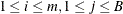
This function computes the limited moment of order
with upper limit for any continuous probability distribution. The limited moment is defined as
![$\displaystyle E[(X \wedge u)^ k] $](images/etshpug_hpseverity0701.png)
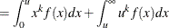

where
 and
and  denote the PDF and the CDF of the distribution, respectively. The LIMMOMENT function uses the following alternate definition,
which can be derived using integration-by-parts:
denote the PDF and the CDF of the distribution, respectively. The LIMMOMENT function uses the following alternate definition,
which can be derived using integration-by-parts:
![\[ E[(X \wedge u)^ k] = k \int _{0}^{u} (1-F(x)) x^{k-1} dx \]](images/etshpug_hpseverity0707.png)
You need to specify the CDF function of the distribution, the values of its parameters, and the values of
and to compute the limited moment.