The MCMC Procedure
-
Overview

-
Getting Started
-
Syntax
-
Details
How PROC MCMC Works Blocking of Parameters Sampling Methods Tuning the Proposal Distribution Conjugate Sampling Initial Values of the Markov Chains Assignments of Parameters Standard Distributions Usage of Multivariate Distributions Specifying a New Distribution Using Density Functions in the Programming Statements Truncation and Censoring Some Useful SAS Functions Matrix Functions in PROC MCMC Create Design Matrix Modeling Joint Likelihood Regenerating Diagnostics Plots Caterpillar Plot Posterior Predictive Distribution Handling of Missing Data Floating Point Errors and Overflows Handling Error Messages Computational Resources Displayed Output ODS Table Names ODS Graphics
-
Examples
Simulating Samples From a Known Density Box-Cox Transformation Logistic Regression Model with a Diffuse Prior Logistic Regression Model with Jeffreys’ Prior Poisson Regression Nonlinear Poisson Regression Models Logistic Regression Random-Effects Model Nonlinear Poisson Regression Random-Effects Model Multivariate Normal Random-Effects Model Change Point Models Exponential and Weibull Survival Analysis Time Independent Cox Model Time Dependent Cox Model Piecewise Exponential Frailty Model Normal Regression with Interval Censoring Constrained Analysis Implement a New Sampling Algorithm Using a Transformation to Improve Mixing Gelman-Rubin Diagnostics
- References
Example 54.5 Poisson Regression
You can use the Poisson distribution to model the distribution of cell counts in a multiway contingency table. Aitkin et al. (1989) have used this method to model insurance claims data. Suppose the following hypothetical insurance claims data are classified by two factors: age group (with two levels) and car type (with three levels). The following statements create the data set:
title 'Poisson Regression';
data insure;
   input n c car $ age;
   ln = log(n);
   datalines;
   500   42  small  0
   1200  37  medium 0
   100    1  large  0
   400  101  small  1
   500   73  medium 1
   300   14  large  1
   ;

proc transreg data=insure design;
   model class(car / zero=last);
   id n c age ln;
   output out=input_insure(drop=_: Int:);
   run;
The variable n represents the number of insurance policy holders and the variable c represents the number of insurance claims. The variable car is the type of car involved (classified into three groups), and it is coded into two levels. The variable age is the age group of a policy holder (classified into two groups).
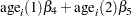
Assume that the number of claims c has a Poisson probability distribution and that its mean,  , is related to the factors car and age for observation
  by
by
 |
 |
 |
|||
 |
|
 |
|||
|
|
 |
|||
|
|
 |
The indicator variables  is associated with the
  th level of the variable car for observation in the following way:
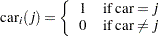 |
A similar coding applies to age. The  ’s are parameters. The logarithm of the variable n is used as an offset—that is, a regression variable with a constant coefficient of 1 for each observation. Having the offset constant in the model is equivalent to fitting an expanded data set with 3000 observations, each with response variable y observed on an individual level. The log link relates the mean and the factors car and age.
The following statements run PROC MCMC:
proc mcmc data=input_insure outpost=insureout nmc=5000 propcov=quanew
          maxtune=0 seed=7;
   ods select PostSummaries PostIntervals;
   array data[4] 1 &_trgind age;
   array beta[4] alpha beta_car1 beta_car2 beta_age;
   parms alpha beta:;
   prior alpha beta: ~ normal(0, prec = 1e-6);
   call mult(data, beta, mu);
   model c ~ poisson(exp(mu+ln));
run;
The analysis uses a relatively flat prior on all the regression coefficients, with mean at  and precision at
  . The option MAXTUNE=0 skips the tuning phase because the optimization routine (PROPCOV=QUANEW) provides good initial values and proposal covariance matrix.
There are four parameters in the model: alpha is the intercept; beta_car1 and beta_car2 are coefficients for the class variable car, which has three levels; and beta_age is the coefficient for age. The symbol mu connects the regression model and the Poisson mean by using the log link. The MODEL statement specifies a Poisson likelihood for the response variable c.
Posterior summary and interval statistics are shown in Output 54.5.1.
| Poisson Regression |
| Posterior Summaries | ||||||
|---|---|---|---|---|---|---|
| Parameter | N | Mean | Standard Deviation |
Percentiles | ||
| 25% | 50% | 75% | ||||
| alpha | 5000 | -2.6403 | 0.1344 | -2.7261 | -2.6387 | -2.5531 |
| beta_car1 | 5000 | -1.8335 | 0.2917 | -2.0243 | -1.8179 | -1.6302 |
| beta_car2 | 5000 | -0.6931 | 0.1255 | -0.7775 | -0.6867 | -0.6118 |
| beta_age | 5000 | 1.3151 | 0.1386 | 1.2153 | 1.3146 | 1.4094 |
| Posterior Intervals | |||||
|---|---|---|---|---|---|
| Parameter | Alpha | Equal-Tail Interval | HPD Interval | ||
| alpha | 0.050 | -2.9201 | -2.3837 | -2.9133 | -2.3831 |
| beta_car1 | 0.050 | -2.4579 | -1.3036 | -2.4692 | -1.3336 |
| beta_car2 | 0.050 | -0.9462 | -0.4497 | -0.9485 | -0.4589 |
| beta_age | 0.050 | 1.0442 | 1.5898 | 1.0387 | 1.5812 |
To fit the same model by using PROC GENMOD, you can do the following. Note that the default normal prior on the coefficients is 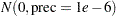 , the same as used in the PROC MCMC. The following statements run PROC GENMOD and create Output 54.5.2:
proc genmod data=insure;
   ods select PostSummaries PostIntervals;
   class car age(descending);
   model c = car age / dist=poisson link=log offset=ln;
   bayes seed=17 nmc=5000 coeffprior=normal;
run;
To compare, posterior summary and interval statistics from PROC GENMOD are reported in Output 54.5.2, and they are very similar to PROC MCMC results in Output 54.5.1.
| Poisson Regression |
| Posterior Summaries | ||||||
|---|---|---|---|---|---|---|
| Parameter | N | Mean | Standard Deviation |
Percentiles | ||
| 25% | 50% | 75% | ||||
| Intercept | 5000 | -2.6353 | 0.1299 | -2.7243 | -2.6312 | -2.5455 |
| carlarge | 5000 | -1.7996 | 0.2752 | -1.9824 | -1.7865 | -1.6139 |
| carmedium | 5000 | -0.6977 | 0.1269 | -0.7845 | -0.6970 | -0.6141 |
| age1 | 5000 | 1.3148 | 0.1348 | 1.2237 | 1.3138 | 1.4067 |
| Posterior Intervals | |||||
|---|---|---|---|---|---|
| Parameter | Alpha | Equal-Tail Interval | HPD Interval | ||
| Intercept | 0.050 | -2.8952 | -2.3867 | -2.8755 | -2.3730 |
| carlarge | 0.050 | -2.3538 | -1.2789 | -2.3424 | -1.2691 |
| carmedium | 0.050 | -0.9494 | -0.4487 | -0.9317 | -0.4337 |
| age1 | 0.050 | 1.0521 | 1.5794 | 1.0624 | 1.5863 |
Note that the descending option in the CLASS statement reverses the sorting order of the class variable age so that the results agree with PROC MCMC. If this option is not used, the estimate for age has a reversed sign as compared to Output 54.5.2.