The MCMC Procedure

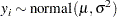
Conjugate prior is a family of prior distributions in which the prior and the posterior distributions are of the same family of distributions. For example, if you model an independently and identically distributed random variable using a normal likelihood with known variance ,

a normal prior on

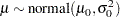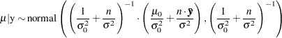
is a conjugate prior because the posterior distribution of is also a normal distribution given , , , and :

Conjugate sampling is efficient because it enables the Markov chain to obtain samples from the target distribution directly. When appropriate, PROC MCMC uses conjugate sampling methods to draw conditional posterior samples. Table 54.6 lists scenarios that lead to conjugate sampling in PROC MCMC.

In most cases, Family in Output 54.6 refers to the likelihood function. However, it does not necessarily have to be the case. The Family is a distribution that is conditional on the parameter of interest, and it can appear in any level of the hierarchical model, including on the random-effects level.

PROC MCMC can detect conjugacy only if the model parameter (not a function or a transformation of the model parameter) is used in the prior and Family distributions. For example, the following program leads to a conjugate sampler being used on the parameter mu:

parm mu;
prior mu ~ n(0, sd=1000);
model y ~ n(mu, var=s2);

However, if you modify the program slightly in the following way, although the conjugacy still holds in theory, PROC MCMC cannot detect conjugacy on mu because the parameter enters the normal likelihood function through the symbol w:

parm mu;
prior mu ~ n(0, sd=1000);
w = mu;
model y ~ n(w, var=s2);

In this case, PROC MCMC resorts to the default sampling algorithm, which is a random walk Metropolis based on a normal kernel.

Similarly, the following statements also prevent PROC MCMC from detecting conjugacy on the parameter mu:

parm mu;
prior mu ~ n(0, sd=1000);
model y ~ n(mu + 2, var=s2);

When conjugacy is defected in a model, PROC MCMC performs a numerical optimization on the joint posterior distribution at the start of the MCMC simulation. To turn off this pre-optimization routine, use option PROPCOV=IND.

In a normal family, an often-used conjugate prior on the variance is

igamma(shape=0.001, scale=0.001)

An often-used conjugate prior on the precision is

gamma(shape=0.001, iscale=0.001)

You want to exercise caution in using the igamma and gamma distributions as PROC MCMC suports both scale and iscale parametrizations in these distributions.