The MCMC Procedure
-
Overview

-
Getting Started
-
Syntax
-
Details
How PROC MCMC Works Blocking of Parameters Sampling Methods Tuning the Proposal Distribution Conjugate Sampling Initial Values of the Markov Chains Assignments of Parameters Standard Distributions Usage of Multivariate Distributions Specifying a New Distribution Using Density Functions in the Programming Statements Truncation and Censoring Some Useful SAS Functions Matrix Functions in PROC MCMC Create Design Matrix Modeling Joint Likelihood Regenerating Diagnostics Plots Caterpillar Plot Posterior Predictive Distribution Handling of Missing Data Floating Point Errors and Overflows Handling Error Messages Computational Resources Displayed Output ODS Table Names ODS Graphics
-
Examples
Simulating Samples From a Known Density Box-Cox Transformation Logistic Regression Model with a Diffuse Prior Logistic Regression Model with Jeffreys’ Prior Poisson Regression Nonlinear Poisson Regression Models Logistic Regression Random-Effects Model Nonlinear Poisson Regression Random-Effects Model Multivariate Normal Random-Effects Model Change Point Models Exponential and Weibull Survival Analysis Time Independent Cox Model Time Dependent Cox Model Piecewise Exponential Frailty Model Normal Regression with Interval Censoring Constrained Analysis Implement a New Sampling Algorithm Using a Transformation to Improve Mixing Gelman-Rubin Diagnostics
- References
| Random-Effects Model |
This example illustrates how you can fit a normal likelihood random-effects model in PROC MCMC. PROC MCMC offers you the ability to model beyond the normal likelihood (see Logistic Regression Random-Effects Model, Nonlinear Poisson Regression Random-Effects Model, and Piecewise Exponential Frailty Model).
Consider a scenario in which data are collected in groups and you want to model group-specific effects. You can use a random-effects model (sometimes also known as a variance-components model):
 |
where  is the group index and
  indexes the observations in the
  th group. In the regression model, the fixed effects
  and
and  are the intercept and the coefficient for variable
  , respectively. The random effect
  is the mean for the th group, and
  are the error term.
Consider the following SAS data set:
title 'Random-Effects Model';

data heights;
   input Family G$ Height @@;
   datalines;
1 F 67   1 F 66   1 F 64   1 M 71   1 M 72   2 F 63
2 F 63   2 F 67   2 M 69   2 M 68   2 M 70   3 F 63
3 M 64   4 F 67   4 F 66   4 M 67   4 M 67   4 M 69
;
The response variable Height measures the heights (in inches) of 18 individuals. The covariate  is the gender (variable G), and the individuals are grouped according to Family (group index). Since the variable G is a character variable and PROC MCMC does not support a CLASS statement, you need to create the corresponding design matrix. In this example, the design matrix for a factor variable of level 2 (M and F) can be constructed using the following statement:
data input;
   set heights;
   if g eq 'F' then gf = 1;
   else gf = 0;
   drop g;
run;
The data set variable gf is a numeric variable and can be used in the regression model in PROC MCMC.
In data sets with factor variables that have more levels, you can consider using PROC TRANSREG to construct the design matrix. See the section Create Design Matrix for more information.
To model the data, you can assume that Height is normally distributed:
 |
The priors on the parameters , , are also assumed to be normal:
 |
 |
 |
|||
 |
|
|
|||
 |
|
 |
Priors on the variance terms,  and
and  , are inverse-gamma:
 |
|
 |
|||
 |
|
|
The inverse-gamma distribution is a conjugate prior for the variance in the normal likelihood and the variance in the prior distribution of the random effect.
The following statements fit a linear random-effects model to the data and produce the output shown in Figure 54.10 and Figure 54.11:
ods graphics on;
proc mcmc data=input outpost=postout nmc=50000 thin=5 seed=7893;
ods select Parameters REparameters PostSummaries PostIntervals
tadpanel;
parms b0 0 b1 0 s2 1 s2g 1;
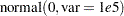
prior b: ~ normal(0, var = 10000);
prior s: ~ igamma(0.01, scale = 0.01);
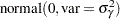
random gamma ~ normal(0, var = s2g) subject=family monitor=(gamma);
mu = b0 + b1 * gf + gamma;
model height ~ normal(mu, var = s2);
run;
ods graphics off;
Some of the statements are very similar to those shown in the previous two examples. The ODS GRAPHICS ON statement enables ODS Graphics. The PROC MCMC statement specifies the input and output data sets, the simulation size, the thinning rate, and a random number seed. The ODS SELECT statement displays the model parameter and random-effects parameter information tables, summary statistics table, the interval statistics table, and the diagnostics plots.
The PARMS statement lumps all four model parameters in a single block. They are b0 (overall intercept), b1 (main effect for gf), s2 (variance of the likelihood function), and s2g (variance of the random effect). If a random walk Metropolis sampler is the only applicable sampler for all parameters, then these four parameters are updated in a single block. However, since the conjugate updater is used to draw posterior samples of s2 and s2g, PROC MCMC updates these parameters separately (see the Block column in "Parameters" table in Figure 54.9).
The PRIOR statements specify priors for all the parameters. The notation b: is a shorthand for all symbols that start with the letter ‘b’. In this example, b: includes b0 and b1. Similarly, s: stands for both s2 and s2g. This shorthand notation can save you some typing, and it keeps your statements tidy.
The RANDOM statement specifies a single random effect to be gamma, and specifies that it has a normal prior centered at 0 with variance s2g. The SUBJECT= argument in the RANDOM statement defines a group index (family) in the model, where all observations from the same family should have the same group indicator value. The MONITOR= option outputs analysis for all the random-effects parameters.
Finally, the mu assignment statement calculates the expected value of height in the random-effects model. The MODEL statement specifies the likelihood function for height.
The "Parameters" and "Random-Effects Parameters" tables, shown in Figure 54.9, contain information about the model parameters and the four random-effects parameters.
| Random-Effects Model |
| Parameters | ||||
|---|---|---|---|---|
| Block | Parameter | Sampling Method |
Initial Value |
Prior Distribution |
| 1 | s2 | Conjugate | 1.0000 | igamma(0.01, scale = 0.01) |
| 2 | s2g | Conjugate | 1.0000 | igamma(0.01, scale = 0.01) |
| 3 | b0 | N-Metropolis | 0 | normal(0, var = 10000) |
| b1 | 0 | normal(0, var = 10000) | ||
| Random Effects Parameters | |||
|---|---|---|---|
| Parameter | Subject | Levels | Prior Distribution |
| gamma | Family | 4 | normal(0, var = s2g) |
The posterior summary and interval statistics for b0 and b1 are shown in Figure 54.10.
| Random-Effects Model |
| Posterior Summaries | ||||||
|---|---|---|---|---|---|---|
| Parameter | N | Mean | Standard Deviation |
Percentiles | ||
| 25% | 50% | 75% | ||||
| b0 | 10000 | 68.4591 | 1.2085 | 67.7939 | 68.4369 | 69.0863 |
| b1 | 10000 | -3.5381 | 0.9622 | -4.1439 | -3.5351 | -2.9466 |
| s2 | 10000 | 4.1495 | 1.9089 | 2.8251 | 3.7353 | 4.9854 |
| s2g | 10000 | 4.8368 | 17.4110 | 0.2218 | 1.2534 | 4.0669 |
| gamma_1 | 10000 | 0.9374 | 1.2817 | 0.0832 | 0.6802 | 1.6250 |
| gamma_2 | 10000 | 0.0167 | 1.1399 | -0.4145 | 0.0325 | 0.5038 |
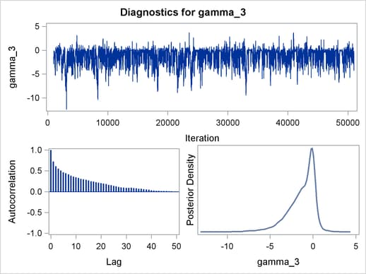
| gamma_3 | 10000 | -1.3313 | 1.6080 | -2.1514 | -0.9247 | -0.1434 |
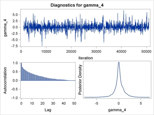
| gamma_4 | 10000 | 0.0979 | 1.1495 | -0.3470 | 0.0537 | 0.5802 |
| Posterior Intervals | |||||
|---|---|---|---|---|---|
| Parameter | Alpha | Equal-Tail Interval | HPD Interval | ||
| b0 | 0.050 | 66.0454 | 71.1125 | 65.8787 | 70.7985 |
| b1 | 0.050 | -5.4303 | -1.5336 | -5.4941 | -1.6259 |
| s2 | 0.050 | 1.7532 | 9.0102 | 1.4424 | 8.0066 |
| s2g | 0.050 | 0.0117 | 29.7402 | 0.00121 | 18.3336 |
| gamma_1 | 0.050 | -1.1857 | 3.8472 | -1.1522 | 3.8666 |
| gamma_2 | 0.050 | -2.6485 | 2.4385 | -2.3792 | 2.6240 |
| gamma_3 | 0.050 | -5.4020 | 0.6187 | -4.8669 | 0.8624 |
| gamma_4 | 0.050 | -2.5324 | 2.6004 | -2.2341 | 2.7602 |
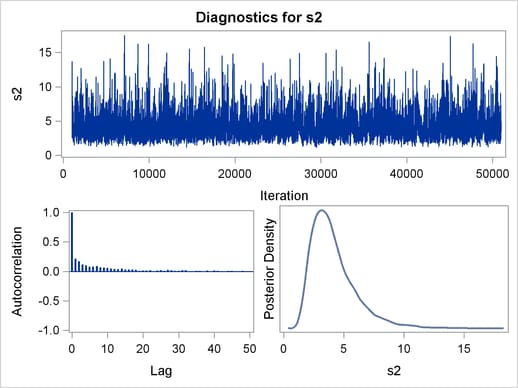
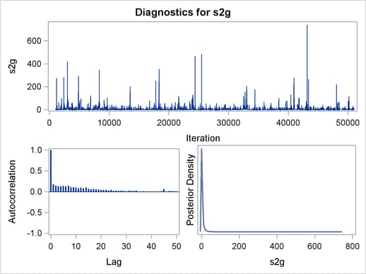
Trace plots, autocorrelation plots, and posterior density plots for all the parameters are shown in Figure 54.11. The mixing looks very reasonable, suggesting convergence.
 and Log of the Posterior Density
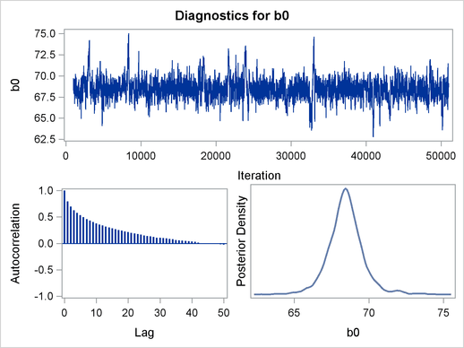
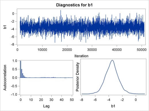
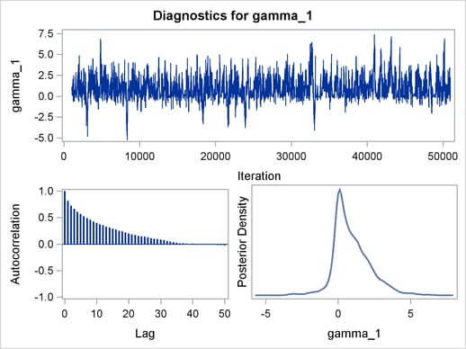
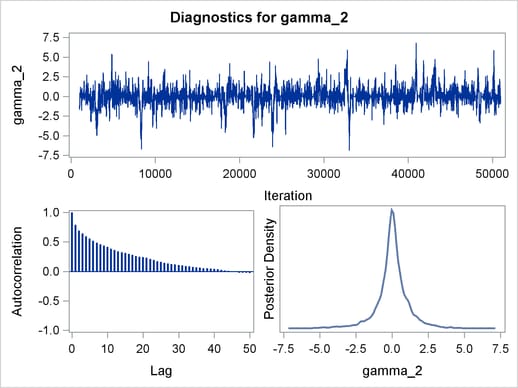
From the interval statistics table, you see that both the equal-tail and HPD intervals for are positive, strongly indicating the positive effect of the parameter. On the other hand, both intervals for cover the value zero, indicating that gf does not have a strong impact on predicting height in this model.