The GLMSELECT Procedure
-
Overview

- Getting Started
-
Syntax
-
Details
Model-Selection Methods Model Selection Issues Criteria Used in Model Selection Methods CLASS Variable Parameterization and the SPLIT Option Macro Variables Containing Selected Models Using the STORE Statement Building the SSCP Matrix Model Averaging Using Validation and Test Data Cross Validation Displayed Output ODS Table Names ODS Graphics
-
Examples
- References
Example 44.5 Model Averaging
This example shows how you can combine variable selection methods with model averaging to build parsimonious predictive models. This example uses simulated data that consist of observations from the model
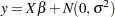 |
where  is drawn from a multivariate normal distribution
  with
with  where
where  . This setup has been widely studied in investigations of variable selection methods. For examples, see Breiman (1992), Tibshirani (1996), and Zou (2006).
The following statements define a macro that uses the SIMNORMAL procedure to generate the regressors. This macro prepares a TYPE=CORR data set that specifies the desired pairwise correlations. This data set is used as the input data for PROC SIMNORMAL which produces the sampled regressors in an output data set named Regressors.
%macro makeRegressorData(nObs=100,nVars=8,rho=0.5,seed=1);
   data varCorr;
     drop i j;
     array x{&nVars};
     length  _NAME_ $8   _TYPE_ $8;
     _NAME_ = '';

     _TYPE_ = 'MEAN';
     do j=1 to &nVars; x{j}=0; end;
     output;

     _TYPE_ = 'STD';
     do j=1 to &nVars; x{j}=1;end;
     output;

     _TYPE_ = 'N';
     do j=1 to &nVars; x{j}=10000;end;
     output;

     _TYPE_ = 'CORR';
     do i=1 to &nVars;
        _NAME_="x" || trim(left(i));
        do j= 1 to &nVars;
           x{j}=&rho**(abs(i-j));
        end;
        output;
     end;
   run;

   proc simnormal data=varCorr(type=corr) out=Regressors
               numReal=&nObs seed=&seed;
      var x1-x&nVars;
   run;
%mend;
The following statements use the %makeRegressorData macro to generate a sample of 100 observations with 10 regressors, where 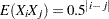 , the true coefficients are
  , and
, and  .
.
%makeRegressorData(nObs=100,nVars=10,rho=0.5);

data simData;
    set regressors;
    yTrue = 3*x1 + 1.5*x2 + 2*x5;
    y     = yTrue + 3*rannor(2);
run;
The adaptive lasso algorithm (see Adaptive Lasso Selection) is a modification of the standard lasso algorithm in which weights are applied to each of the parameters in forming the lasso constraint. Zou (2006) shows that the adaptive lasso has theoretical advantages over the standard lasso. Furthermore, simulation studies show that the adaptive lasso tends to perform better than the standard lasso in selecting the correct regressors, particularly in high signal-to-noise ratio cases. The following statements fit an adaptive lasso model to the simData data:
proc glmselect data=simData;
   model y=x1-x10/selection=LASSO(adaptive stop=none choose=sbc);
run;
The selected model and parameter estimates are shown in Output 44.5.1
| Effects: | Intercept x1 x2 x5 |
|---|
| Parameter Estimates | ||
|---|---|---|
| Parameter | DF | Estimate |
| Intercept | 1 | -0.243219 |
| x1 | 1 | 3.246129 |
| x2 | 1 | 1.310514 |
| x5 | 1 | 2.132416 |
You see that the selected model contains only the relevant regressors x1, x2, and x5. You might want to investigate how frequently the adaptive lasso method selects just the relevant regressors and how stable the corresponding parameter estimates are. In a simulation study, you can do this by drawing new samples and repeating this process many times. What can you do when you only have a single sample of the data available? One approach is to repeatedly draw subsamples from the data that you have, and to fit models for each of these samples. You can then form the average model and use this model for prediction. You can also examine how frequently models are selected, and you can use the frequency of effect selection as a measure of effect importance.
The following statements show how you can use the MODELAVERAGE statement to perform such an analysis:
ods graphics on;

proc glmselect data=simData seed=3 plots=(EffectSelectPct ParmDistribution);
   model y=x1-x10/selection=LASSO(adaptive stop=none choose=SBC);
   modelAverage tables=(EffectSelectPct(all) ParmEst(all));
run;
The "ModelAverageInfo" table in Output 44.5.2 shows that the default sampling method is the bootstrap approach of drawing 100 samples with replacement, where the sampling percentage of 100 means that each sample has the same sum of frequencies as the input data. You can use the SAMPLING= and NSAMPLES= options in the MODELAVERAGE statement to modify the sampling method and the number of samples used.
| Model Averaging Information | |
|---|---|
| Sampling Method | Unrestricted (with replacement) |
| Sample Percentage | 100 |
| Number of Samples | 100 |
Output 44.5.3 shows the percentage of samples where each effect is in the selected model. The ALL option of the EFFECTSELECTPCT request in the TABLES= option specifies that effects that appear in any selected model are shown. (By default, the "Effect Selection Percentage" table displays only those effects that are selected at least 20 percent of the time.)
| Effect Selection Percentage |
|
|---|---|
| Effect | Selection Percentage |
| x1 | 100.0 |
| x2 | 99.00 |
| x3 | 33.00 |
| x4 | 7.00 |
| x5 | 100.0 |
| x6 | 14.00 |
| x7 | 25.00 |
| x8 | 9.00 |
| x9 | 7.00 |
| x10 | 16.00 |
The EFFECTSELECTPCT request in the PLOTS= option in the PROC GLMSELECT statement produces the bar chart shown in Output 44.5.4, which graphically displays the information in the "EffectSelectPct" table.
Output 44.5.5 shows the frequencies with which models get selected. By default, only the "best" 20 models are shown. See the section Model Selection Frequencies and Frequency Scores for details about how these models are ordered.
| Model Selection Frequency | ||||
|---|---|---|---|---|
| Times Selected | Selection Percentage |
Number of Effects | Frequency Score |
Effects in Model |
| 44 | 44.00 | 4 | 45.00 | Intercept x1 x2 x5 |
| 9 | 9.00 | 5 | 9.86 | Intercept x1 x2 x3 x5 |
| 8 | 8.00 | 6 | 8.76 | Intercept x1 x2 x3 x5 x7 |
| 4 | 4.00 | 5 | 4.82 | Intercept x1 x2 x5 x8 |
| 4 | 4.00 | 7 | 4.67 | Intercept x1 x2 x3 x5 x6 x7 |
| 3 | 3.00 | 5 | 3.85 | Intercept x1 x2 x5 x7 |
| 2 | 2.00 | 5 | 2.83 | Intercept x1 x2 x5 x10 |
| 2 | 2.00 | 5 | 2.81 | Intercept x1 x2 x4 x5 |
| 2 | 2.00 | 6 | 2.74 | Intercept x1 x2 x3 x5 x6 |
| 2 | 2.00 | 7 | 2.66 | Intercept x1 x2 x3 x5 x6 x10 |
| 1 | 1.00 | 5 | 1.83 | Intercept x1 x2 x5 x6 |
| 1 | 1.00 | 4 | 1.81 | Intercept x1 x5 x7 |
| 1 | 1.00 | 5 | 1.81 | Intercept x1 x2 x5 x9 |
| 1 | 1.00 | 6 | 1.75 | Intercept x1 x2 x3 x5 x10 |
| 1 | 1.00 | 6 | 1.74 | Intercept x1 x2 x3 x5 x8 |
| 1 | 1.00 | 6 | 1.73 | Intercept x1 x2 x5 x6 x7 |
| 1 | 1.00 | 6 | 1.72 | Intercept x1 x2 x5 x7 x9 |
| 1 | 1.00 | 6 | 1.71 | Intercept x1 x2 x5 x8 x10 |
| 1 | 1.00 | 6 | 1.70 | Intercept x1 x2 x4 x5 x10 |
| 1 | 1.00 | 7 | 1.68 | Intercept x1 x2 x3 x5 x7 x10 |
You can see that the most frequently selected model is the model that contains just the true underlying regressors. Although this model is selected in 44% of the samples, most of the selected models contain at least one irrelevant regressor. This is not surprising because even though the true model has just a few large effects in this example, the regressors have nontrivial pairwise correlations.
When your goal is simply to obtain a predictive model, then a good strategy is to average the predictions that you get from all the selected models. In the linear model context, this corresponds to using the model whose parameter estimates are the averages of the estimates that you get for each sample, where if a parameter is not in a selected model, the corresponding estimate is defined to be zero. This has the effect of shrinking the estimates of infrequently selected parameters towards zero.
Output 44.5.6 shows the average parameter estimates. The ALL option of the PARMEST request in the TABLES= option specifies that all parameters that are nonzero in any selected model are shown. (By default, the "Average Parameter Estimates" table displays only those parameters that are nonzero in at least 20 percent of the selected models.)
| Average Parameter Estimates | |||||||
|---|---|---|---|---|---|---|---|
| Parameter | Number Non-zero | Non-zero Percentage | Mean Estimate | Standard Deviation | Estimate Quantiles | ||
| 25% | Median | 75% | |||||
| Intercept | 100 | 100.00 | -0.271262 | 0.308146 | -0.489061 | -0.249163 | -0.058233 |
| x1 | 100 | 100.00 | 3.196392 | 0.377771 | 2.951551 | 3.189078 | 3.446055 |
| x2 | 99 | 99.00 | 1.439966 | 0.416054 | 1.209781 | 1.484064 | 1.710275 |
| x3 | 33 | 33.00 | -0.264831 | 0.412148 | -0.536449 | 0 | 0 |
| x4 | 7 | 7.00 | -0.037810 | 0.142932 | 0 | 0 | 0 |
| x5 | 100 | 100.00 | 2.253196 | 0.397032 | 2.036261 | 2.242240 | 2.489068 |
| x6 | 14 | 14.00 | -0.083823 | 0.261641 | 0 | 0 | 0 |
| x7 | 25 | 25.00 | 0.184656 | 0.372813 | 0 | 0 | 0.143317 |
| x8 | 9 | 9.00 | 0.060438 | 0.206621 | 0 | 0 | 0 |
| x9 | 7 | 7.00 | -0.043307 | 0.239940 | 0 | 0 | 0 |
| x10 | 16 | 16.00 | 0.083411 | 0.199573 | 0 | 0 | 0 |
The average estimate for a parameter is computed by dividing the sum of the estimate values for that parameter in each sample by the total number of samples. This corresponds to using zero as the estimate value for the parameter in those samples where the parameter does not appear in the selected model. Similarly, these zero estimates are included in the computation of the estimated standard deviation and quantiles that are displayed in the "AvgParmEst" table. If you want see the estimates that you get if you do not use zero for nonselected parameters, you can specify the NONZEROPARMS suboption of the PARMEST request in the TABLES=option.
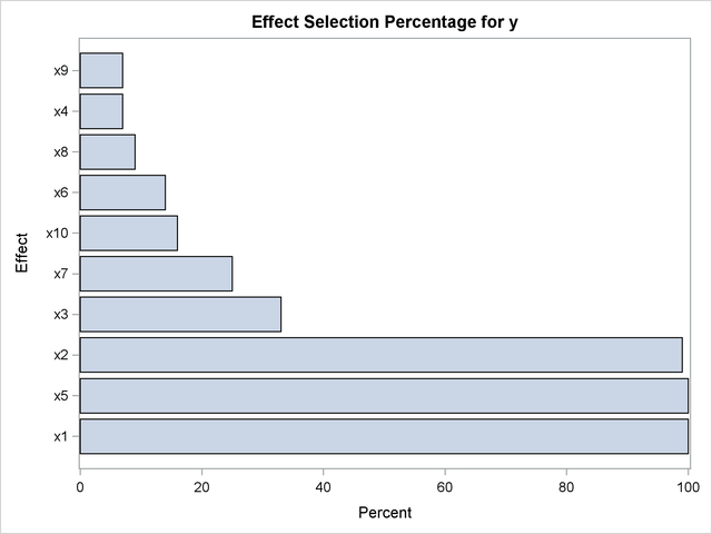
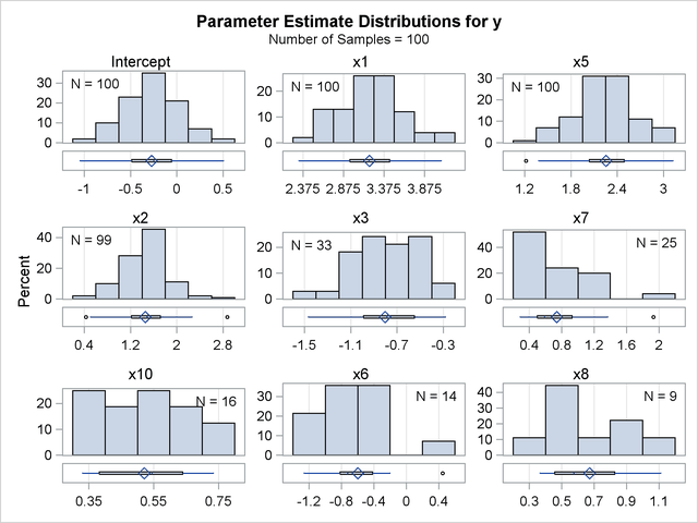
The PARMDISTRIBUTION request in the PLOTS= option in the PROC GLMSELECT statement requests the panel in Output 44.5.7, which shows the distribution of the estimates for each parameter in the average model. For each parameter in the average model, a histogram and box plot of the nonzero values of the estimates are shown. You can use this plot to assess how the selected estimates vary across the samples.
You can obtain details about the model selection for each sample by specifying the DETAILS option in the MODELAVERAGE statement. You can use an OUTPUT statement to output the mean predicted value and standard deviation, quantiles of the predicted values, as well as the individual sample frequencies and predicted values for each sample. The following statements show how you do this:
proc glmselect data=simData seed=3;
   model y=x1-x10/selection=LASSO(adaptive stop=none choose=SBC);
   modelAverage details;
   output out=simOut sampleFreq=sf samplePred=sp
                     p=p stddev=stddev lower=q25 upper=q75 median;
run;
Output 44.5.8 shows the selection summary and parameter estimates for sample 1 of the model averaging. Note that you can obtain all the model selection output, including graphs, for each sample.
| LASSO Selection Summary | ||||
|---|---|---|---|---|
| Step | Effect Entered |
Effect Removed |
Number Effects In |
SBC |
| 0 | Intercept | 1 | 374.8287 | |
| 1 | x1 | 2 | 243.4087 | |
| 2 | x5 | 3 | 227.5991 | |
| 3 | x2 | 4 | 225.7356* | |
| 4 | x7 | 5 | 229.9135 | |
| 5 | x3 | 6 | 233.3660 | |
| 6 | x6 | 7 | 237.7447 | |
| 7 | x10 | 8 | 235.2171 | |
| 8 | x4 | 9 | 238.8085 | |
| 9 | x9 | 10 | 239.8353 | |
| 10 | x8 | 11 | 244.4236 | |
| * Optimal Value Of Criterion | ||||
| Parameter Estimates | ||
|---|---|---|
| Parameter | DF | Estimate |
| Intercept | 1 | -0.092885 |
| x1 | 1 | 4.079938 |
| x2 | 1 | 0.505697 |
| x5 | 1 | 1.473929 |
The following statements display the subset of the variables in the first five observations of the output data set, as shown in Output 44.5.9.
proc print data=simOut(obs=5);
   var p stddev q25 median q75 sf1-sf3 sp1-sp3;
run;
| Obs | p | stddev | q25 | median | q75 | sf1 | sf2 | sf3 | sp1 | sp2 | sp3 |
|---|---|---|---|---|---|---|---|---|---|---|---|
| 1 | 10.3569 | 0.82219 | 9.95992 | 10.3878 | 10.9194 | 1 | 0 | 1 | 10.1378 | 11.2104 | 11.0124 |
| 2 | -5.5453 | 0.64544 | -6.05563 | -5.6455 | -5.0829 | 1 | 1 | 1 | -4.7517 | -6.7191 | -6.4413 |
| 3 | 6.5066 | 0.75289 | 6.05984 | 6.5077 | 6.9099 | 3 | 2 | 0 | 6.0838 | 7.4880 | 6.3466 |
| 4 | -1.7527 | 0.85168 | -2.26638 | -1.8123 | -1.3312 | 1 | 1 | 2 | -2.1891 | -1.4887 | -1.7083 |
| 5 | -7.5840 | 1.20687 | -8.44679 | -7.5716 | -6.7386 | 3 | 1 | 1 | -6.7051 | -9.0558 | -6.7949 |
By default, the LOWER and UPPER options in the OUTPUT statement produce the lower and upper quartiles of the sample predicted values. You can change the quantiles produced by using the ALPHA= option in the MODELAVERAGE statement. The variables sf1–sf100 contain the sample frequencies used for each sample, and the variables sp1–sp100 hold the corresponding predicted values. Even if you do not specify the DETAILS option in the MODELAVERAGE statement, you can use the sample frequencies in the output data set to reproduce the selection results for any particular sample. For example, the following statements recover the selection for sample 1:
proc glmselect data=simOut;
   freq sf1;
   model y=x1-x10/selection=LASSO(adaptive stop=none choose=SBC);
run;
The average model is not parsimonious—it includes shrunken estimates of infrequently selected parameters which often correspond to irrelevant regressors. It is tempting to ignore the estimates of infrequently selected parameters by setting their estimate values to zero in the average model. However, this can lead to a poorly performing model. Even though a parameter might occur in only one selected model, it might be a very important term in that model. Ignoring its estimate but including some of the estimates of the other parameters in this model leads to biased predictions. One scenario where this might occur is when the data contains two highly correlated regressors which are both strongly correlated with the response.
You can obtain a parsimonious model by using the frequency of effect selection as a measure of effect importance and refitting a model that contains just the effects that you deem important. In this example, Output 44.5.3 shows that the effects x1, x2, and x5 all get selected at least 99 percent of the time, whereas all other effects get selected less than 34 percent of the time. This large gap suggests that using 35% as the selection cutoff for this data will produce a parsimonious model that retains good predictive performance. You can use the REFIT option to implement this strategy. The REFIT option requests a second round of model averaging, where you use the MINPCT= suboption to specify the minimum percentage of times an effect must be selected in the initial set of samples to be included in the second round of model averaging. The average model is obtained by averaging the ordinary least squares estimates obtained for each sample. The following statements show how you do this:
proc glmselect data=simData seed=3 plots=(ParmDistribution);
   model y=x1-x10/selection=LASSO(adaptive stop=none choose=SBC);
   modelAverage refit(minpct=35 nsamples=1000) alpha=0.1;
run;

ods graphics off;
The NSAMPLES=1000 suboption of the REFIT option specifies that 1,000 samples be used in the refit, and the MINPCT=35 suboption specifies the cutoff for inclusion in the refit. The ALPHA=0.1 option specifies that the  th and
  th percentiles of the estimates be displayed. Output 44.5.10 shows the effects that are used in performing the refit and the resulting average parameter estimates.
| Effects: | Intercept x1 x2 x5 |
|---|
| Average Parameter Estimates | |||||
|---|---|---|---|---|---|
| Parameter | Mean Estimate | Standard Deviation | Estimate Quantiles | ||
| 5% | Median | 95% | |||
| Intercept | -0.243514 | 0.315207 | -0.762462 | -0.230630 | 0.271510 |
| x1 | 3.226252 | 0.299443 | 2.737843 | 3.226758 | 3.708131 |
| x2 | 1.453584 | 0.308062 | 0.947059 | 1.454635 | 1.968231 |
| x5 | 2.226044 | 0.345185 | 1.627491 | 2.228189 | 2.780034 |
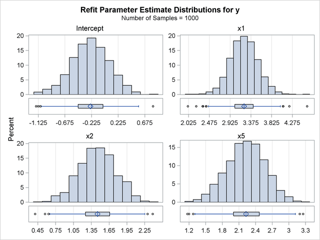
Output 44.5.11 displays the distributions of the estimates that are obtained for each parameter in the refit model. Because the distributions are approximately normal and a large number of samples are used, it is reasonable to interpret the range between the th and th percentiles of each estimate as an approximate 90% confidence interval for that estimate.