The GLMSELECT Procedure
-
Overview

- Getting Started
-
Syntax
-
Details
Model-Selection Methods Model Selection Issues Criteria Used in Model Selection Methods CLASS Variable Parameterization and the SPLIT Option Macro Variables Containing Selected Models Using the STORE Statement Building the SSCP Matrix Model Averaging Using Validation and Test Data Cross Validation Displayed Output ODS Table Names ODS Graphics
-
Examples
- References
Example 44.2 Using Validation and Cross Validation
This example shows how you can use both test set and cross validation to monitor and control variable selection. It also demonstrates the use of split classification variables.
The following statements produce analysis and test data sets. Note that the same statements are used to generate the observations that are randomly assigned for analysis and test roles in the ratio of approximately two to one.
 data analysisData testData;
    drop i j c3Num;
    length c3$ 7;

    array x{20} x1-x20;

    do i=1 to 1500;
       do j=1 to 20;
          x{j} = ranuni(1);
       end;

       c1 = 1 + mod(i,8);
       c2 = ranbin(1,3,.6);

       if      i < 50   then do; c3 = 'tiny';     c3Num=1;end;
       else if i < 250  then do; c3 = 'small';    c3Num=1;end;
       else if i < 600  then do; c3 = 'average';  c3Num=2;end;
       else if i < 1200 then do; c3 = 'big';      c3Num=3;end;
       else                  do; c3 = 'huge';     c3Num=5;end;

       y = 10 + x1 + 2*x5 + 3*x10 + 4*x20  + 3*x1*x7 + 8*x6*x7
              + 5*(c1=3)*c3Num + 8*(c1=7)  + 5*rannor(1);

       if ranuni(1) < 2/3 then output analysisData;
                          else output testData;
   end;
 run;
Suppose you suspect that the dependent variable depends on both main effects and two-way interactions. You can use the following statements to select a model:
ods graphics on;

proc glmselect data=analysisData testdata=testData
               seed=1 plots(stepAxis=number)=(criterionPanel ASEPlot);
   partition fraction(validate=0.5);
   class c1 c2 c3(order=data);
   model y =  c1|c2|c3|x1|x2|x3|x4|x5|x5|x6|x7|x8|x9|x10
             |x11|x12|x13|x14|x15|x16|x17|x18|x19|x20 @2
           / selection=stepwise(choose = validate
                                select = sl)
             hierarchy=single stb;
run;
Note that a TESTDATA= data set is named in the PROC GLMSELECT statement and that a PARTITION statement is used to randomly assign half the observations in the analysis data set for model validation and the rest for model training. You find details about the number of observations used for each role in the number of observations tables shown in Output 44.2.1.
| Observation Profile for Analysis Data | |
|---|---|
| Number of Observations Read | 1010 |
| Number of Observations Used | 1010 |
| Number of Observations Used for Training | 510 |
| Number of Observations Used for Validation | 500 |
The "Class Level Information" and "Dimensions" tables are shown in Output 44.2.2. The "Dimensions" table shows that at each step of the selection process, 278 effects are considered as candidates for entry or removal. Since several of these effects have multilevel classification variables as members, there are 661 parameters.
| Class Level Information | ||
|---|---|---|
| Class | Levels | Values |
| c1 | 8 | 1 2 3 4 5 6 7 8 |
| c2 | 4 | 0 1 2 3 |
| c3 | 5 | tiny small average big huge |
| Dimensions | |
|---|---|
| Number of Effects | 278 |
| Number of Parameters | 661 |
The model statement options request stepwise selection with the default entry and stay significance levels used for both selecting entering and departing effects and stopping the selection method. The CHOOSE=VALIDATE suboption specifies that the selected model is chosen to minimize the predicted residual sum of squares when the models at each step are scored on the observations reserved for validation. The HIERARCHY=SINGLE option specifies that interactions can enter the model only if the corresponding main effects are already in the model, and that main effects cannot be dropped from the model if an interaction with such an effect is in the model. These settings are listed in the model information table shown in Output 44.2.3.
| Data Set | WORK.ANALYSISDATA |
|---|---|
| Test Data Set | WORK.TESTDATA |
| Dependent Variable | y |
| Selection Method | Stepwise |
| Select Criterion | Significance Level |
| Stop Criterion | Significance Level |
| Choose Criterion | Validation ASE |
| Entry Significance Level (SLE) | 0.15 |
| Stay Significance Level (SLS) | 0.15 |
| Effect Hierarchy Enforced | Single |
| Random Number Seed | 1 |
The stop reason and stop details tables are shown in Output 44.2.4. Note that because the STOP= suboption of the SELECTION= option was not explicitly specified, the stopping criterion used is the selection criterion, namely significance level.
| Selection stopped because the candidate for entry has SLE > 0.15 and the candidate for removal has SLS < 0.15. |
| Stop Details | |||||
|---|---|---|---|---|---|
| Candidate For |
Effect | Candidate Significance |
Compare Significance |
||
| Entry | x2*x5 | 0.1742 | > | 0.1500 | (SLE) |
| Removal | x5*x10 | 0.0534 | < | 0.1500 | (SLS) |
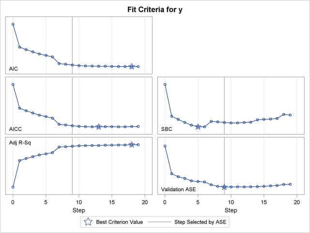
The criterion panel in Output 44.2.5 shows how the various fit criteria evolved as the stepwise selection method proceeded. Note that other than the ASE evaluated on the validation data, these criteria are evaluated on the training data. You see that the minimum of the validation ASE occurs at step 9, and hence the model at this step is selected.
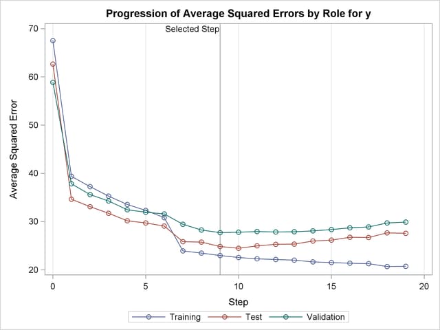
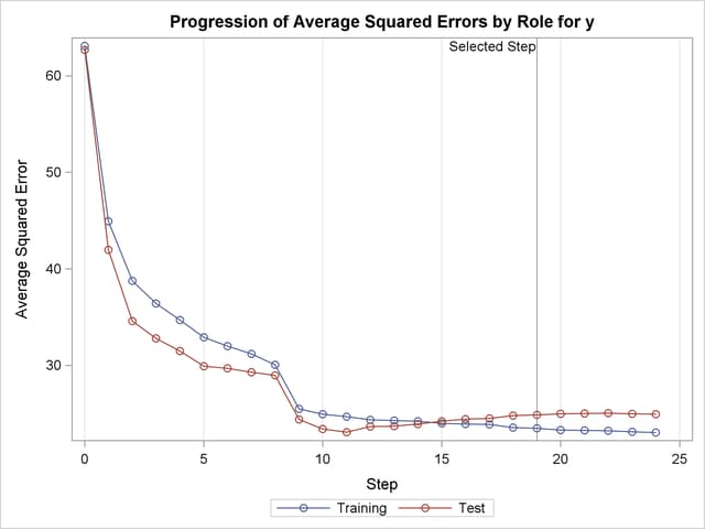
Output 44.2.6 shows how the average squared error (ASE) evolved on the training, validation, and test data. Note that while the ASE on the training data decreases monotonically, the errors on both the validation and test data start increasing beyond step 9. This indicates that models after step 9 are beginning to overfit the training data.
Output 44.2.7 shows the selected effects, analysis of variance, and fit statistics tables for the selected model. Output 44.2.8 shows the parameter estimates table.
| Effects: | Intercept c1 c3 c1*c3 x1 x5 x6 x7 x10 x20 |
|---|
| Analysis of Variance | ||||
|---|---|---|---|---|
| Source | DF | Sum of Squares |
Mean Square |
F Value |
| Model | 44 | 22723 | 516.43621 | 20.49 |
| Error | 465 | 11722 | 25.20856 | |
| Corrected Total | 509 | 34445 | ||
| Root MSE | 5.02081 |
|---|---|
| Dependent Mean | 21.09705 |
| R-Square | 0.6597 |
| Adj R-Sq | 0.6275 |
| AIC | 2200.75319 |
| AICC | 2210.09228 |
| SBC | 1879.30167 |
| ASE (Train) | 22.98427 |
| ASE (Validate) | 27.71105 |
| ASE (Test) | 24.82947 |
| Parameter Estimates | |||||
|---|---|---|---|---|---|
| Parameter | DF | Estimate | Standardized Estimate |
Standard Error | t Value |
| Intercept | 1 | 6.867831 | 0 | 1.524446 | 4.51 |
| c1 1 | 1 | 0.226602 | 0.008272 | 2.022069 | 0.11 |
| c1 2 | 1 | -1.189623 | -0.048587 | 1.687644 | -0.70 |
| c1 3 | 1 | 25.968930 | 1.080808 | 1.693593 | 15.33 |
| c1 4 | 1 | 1.431767 | 0.054892 | 1.903011 | 0.75 |
| c1 5 | 1 | 1.972622 | 0.073854 | 1.664189 | 1.19 |
| c1 6 | 1 | -0.094796 | -0.004063 | 1.898700 | -0.05 |
| c1 7 | 1 | 5.971432 | 0.250037 | 1.846102 | 3.23 |
| c1 8 | 0 | 0 | 0 | . | . |
| c3 tiny | 1 | -2.919282 | -0.072169 | 2.756295 | -1.06 |
| c3 small | 1 | -4.635843 | -0.184338 | 2.218541 | -2.09 |
| c3 average | 1 | 0.736805 | 0.038247 | 1.793059 | 0.41 |
| c3 big | 1 | -1.078463 | -0.063580 | 1.518927 | -0.71 |
| c3 huge | 0 | 0 | 0 | . | . |
| c1*c3 1 tiny | 1 | -2.449964 | -0.018632 | 4.829146 | -0.51 |
| c1*c3 1 small | 1 | 5.265031 | 0.069078 | 3.470382 | 1.52 |
| c1*c3 1 average | 1 | -3.489735 | -0.064365 | 2.850381 | -1.22 |
| c1*c3 1 big | 1 | 0.725263 | 0.017929 | 2.516502 | 0.29 |
| c1*c3 1 huge | 0 | 0 | 0 | . | . |
| c1*c3 2 tiny | 1 | 5.455122 | 0.050760 | 4.209507 | 1.30 |
| c1*c3 2 small | 1 | 7.439196 | 0.131499 | 2.982411 | 2.49 |
| c1*c3 2 average | 1 | -0.739606 | -0.014705 | 2.568876 | -0.29 |
| c1*c3 2 big | 1 | 3.179351 | 0.078598 | 2.247611 | 1.41 |
| c1*c3 2 huge | 0 | 0 | 0 | . | . |
| c1*c3 3 tiny | 1 | -19.266847 | -0.230989 | 3.784029 | -5.09 |
| c1*c3 3 small | 1 | -15.578909 | -0.204399 | 3.266216 | -4.77 |
| c1*c3 3 average | 1 | -18.119398 | -0.395770 | 2.529578 | -7.16 |
| c1*c3 3 big | 1 | -10.650012 | -0.279796 | 2.205331 | -4.83 |
| c1*c3 3 huge | 0 | 0 | 0 | . | . |
| c1*c3 4 tiny | 0 | 0 | 0 | . | . |
| c1*c3 4 small | 1 | 4.432753 | 0.047581 | 3.677008 | 1.21 |
| c1*c3 4 average | 1 | -3.976295 | -0.091632 | 2.625564 | -1.51 |
| c1*c3 4 big | 1 | -1.306998 | -0.033003 | 2.401064 | -0.54 |
| c1*c3 4 huge | 0 | 0 | 0 | . | . |
| c1*c3 5 tiny | 1 | 6.714186 | 0.062475 | 4.199457 | 1.60 |
| c1*c3 5 small | 1 | 1.565637 | 0.022165 | 3.182856 | 0.49 |
| c1*c3 5 average | 1 | -4.286085 | -0.068668 | 2.749142 | -1.56 |
| c1*c3 5 big | 1 | -2.046468 | -0.045949 | 2.282735 | -0.90 |
| c1*c3 5 huge | 0 | 0 | 0 | . | . |
| c1*c3 6 tiny | 1 | 5.135111 | 0.039052 | 4.754845 | 1.08 |
| c1*c3 6 small | 1 | 4.442898 | 0.081945 | 3.079524 | 1.44 |
| c1*c3 6 average | 1 | -2.287870 | -0.056559 | 2.601384 | -0.88 |
| c1*c3 6 big | 1 | 1.598086 | 0.043542 | 2.354326 | 0.68 |
| c1*c3 6 huge | 0 | 0 | 0 | . | . |
| c1*c3 7 tiny | 1 | 1.108451 | 0.010314 | 4.267509 | 0.26 |
| c1*c3 7 small | 1 | 7.441059 | 0.119214 | 3.135404 | 2.37 |
| c1*c3 7 average | 1 | 1.796483 | 0.038106 | 2.630570 | 0.68 |
| c1*c3 7 big | 1 | 3.324160 | 0.095173 | 2.303369 | 1.44 |
| c1*c3 7 huge | 0 | 0 | 0 | . | . |
| c1*c3 8 tiny | 0 | 0 | 0 | . | . |
| c1*c3 8 small | 0 | 0 | 0 | . | . |
| c1*c3 8 average | 0 | 0 | 0 | . | . |
| c1*c3 8 big | 0 | 0 | 0 | . | . |
| c1*c3 8 huge | 0 | 0 | 0 | . | . |
| x1 | 1 | 2.713527 | 0.091530 | 0.836942 | 3.24 |
| x5 | 1 | 2.810341 | 0.098303 | 0.816290 | 3.44 |
| x6 | 1 | 4.837022 | 0.167394 | 0.810402 | 5.97 |
| x7 | 1 | 5.844394 | 0.207035 | 0.793775 | 7.36 |
| x10 | 1 | 2.463916 | 0.087712 | 0.794599 | 3.10 |
| x20 | 1 | 4.385924 | 0.156155 | 0.787766 | 5.57 |
The magnitudes of the standardized estimates and the  statistics of the parameters of the effect "c1" reveal that only levels "3" and "7" of this effect contribute appreciably to the model. This suggests that a more parsimonious model with similar or better predictive power might be obtained if parameters corresponding to the levels of "c1" are allowed to enter or leave the model independently. You request this with the SPLIT option in the CLASS statement as shown in the following statements:
proc glmselect data=analysisData testdata=testData
               seed=1 plots(stepAxis=number)=all;
   partition fraction(validate=0.5);
   class c1(split) c2 c3(order=data);
   model y =  c1|c2|c3|x1|x2|x3|x4|x5|x5|x6|x7|x8|x9|x10
             |x11|x12|x13|x14|x15|x16|x17|x18|x19|x20 @2
           / selection=stepwise(stop   = validate
                                select = sl)
             hierarchy=single;
   output out=outData;
run;
The "Class Level Information" and "Dimensions" tables are shown in Output 44.2.9. The "Dimensions" table shows that while the model statement specifies 278 effects, after splitting the parameters corresponding to the levels of "c1," there are 439 split effects that are considered for entry or removal at each step of the selection process. Note that the total number of parameters considered is not affected by the split option.
| Class Level Information | |||
|---|---|---|---|
| Class | Levels | Values | |
| c1 | 8 | * | 1 2 3 4 5 6 7 8 |
| c2 | 4 | 0 1 2 3 | |
| c3 | 5 | tiny small average big huge | |
| * Associated Parameters Split | |||
| Dimensions | |
|---|---|
| Number of Effects | 278 |
| Number of Effects after Splits | 439 |
| Number of Parameters | 661 |
The stop reason and stop details tables are shown in Output 44.2.10. Since the validation ASE is specified as the stopping criterion, the selection stops at step 11, where the validation ASE achieves a local minimum and the model at this step is the selected model.
| Selection stopped at a local minimum of the residual sum of squares of the validation data. |
| Stop Details | ||||
|---|---|---|---|---|
| Candidate For |
Effect | Candidate Validation ASE |
Compare Validation ASE |
|
| Entry | x18 | 25.9851 | > | 25.7462 |
| Removal | x6*x7 | 25.7611 | > | 25.7462 |
You find details of the selected model in Output 44.2.11. The list of selected effects confirms that parameters corresponding to levels "3" and "7" only of "c1" are in the selected model. Notice that the selected model with classification variable "c1" split contains 18 parameters, whereas the selected model without splitting "c1" has 45 parameters. Furthermore, by comparing the fit statistics in Output 44.2.7 and Output 44.2.11, you see that this more parsimonious model has smaller prediction errors on both the validation and test data.
| Effects: | Intercept c1_3 c1_7 c3 c1_3*c3 x1 x5 x6 x7 x6*x7 x10 x20 |
|---|
| Analysis of Variance | ||||
|---|---|---|---|---|
| Source | DF | Sum of Squares |
Mean Square |
F Value |
| Model | 17 | 22111 | 1300.63200 | 51.88 |
| Error | 492 | 12334 | 25.06998 | |
| Corrected Total | 509 | 34445 | ||
| Root MSE | 5.00699 |
|---|---|
| Dependent Mean | 21.09705 |
| R-Square | 0.6419 |
| Adj R-Sq | 0.6295 |
| AIC | 2172.72685 |
| AICC | 2174.27787 |
| SBC | 1736.94624 |
| ASE (Train) | 24.18515 |
| ASE (Validate) | 25.74617 |
| ASE (Test) | 22.57297 |
When you use a PARTITION statement to subdivide the analysis data set, an output data set created with the OUTPUT statement contains a variable named "_ROLE_" that shows the role each observation was assigned to. See the section OUTPUT Statement and the section Using Validation and Test Data for additional details.
The following statements use PROC PRINT to produce Output 44.2.12, which shows the first five observations of the outData data set.
proc print data=outData(obs=5);
run;
| Obs | c3 | x1 | x2 | x3 | x4 | x5 | x6 | x7 | x8 | x9 | x10 | x11 | x12 | x13 | x14 | x15 | x16 | x17 | x18 | x19 | x20 | c1 | c2 | y | _ROLE_ | p_y |
|---|---|---|---|---|---|---|---|---|---|---|---|---|---|---|---|---|---|---|---|---|---|---|---|---|---|---|
| 1 | tiny | 0.18496 | 0.97009 | 0.39982 | 0.25940 | 0.92160 | 0.96928 | 0.54298 | 0.53169 | 0.04979 | 0.06657 | 0.81932 | 0.52387 | 0.85339 | 0.06718 | 0.95702 | 0.29719 | 0.27261 | 0.68993 | 0.97676 | 0.22651 | 2 | 1 | 11.4391 | VALIDATE | 18.5069 |
| 2 | tiny | 0.47579 | 0.84499 | 0.63452 | 0.59036 | 0.58258 | 0.37701 | 0.72836 | 0.50660 | 0.93121 | 0.92912 | 0.58966 | 0.29722 | 0.39104 | 0.47243 | 0.67953 | 0.16809 | 0.16653 | 0.87110 | 0.29879 | 0.93464 | 3 | 1 | 31.4596 | TRAIN | 26.2188 |
| 3 | tiny | 0.51132 | 0.43320 | 0.17611 | 0.66504 | 0.40482 | 0.12455 | 0.45349 | 0.19955 | 0.57484 | 0.73847 | 0.43981 | 0.04937 | 0.52238 | 0.34337 | 0.02271 | 0.71289 | 0.93706 | 0.44599 | 0.94694 | 0.71290 | 4 | 3 | 16.4294 | VALIDATE | 17.0979 |
| 4 | tiny | 0.42071 | 0.07174 | 0.35849 | 0.71143 | 0.18985 | 0.14797 | 0.56184 | 0.27011 | 0.32520 | 0.56918 | 0.04259 | 0.43921 | 0.91744 | 0.52584 | 0.73182 | 0.90522 | 0.57600 | 0.18794 | 0.33133 | 0.69887 | 5 | 3 | 15.4815 | VALIDATE | 16.1567 |
| 5 | tiny | 0.42137 | 0.03798 | 0.27081 | 0.42773 | 0.82010 | 0.84345 | 0.87691 | 0.26722 | 0.30602 | 0.39705 | 0.34905 | 0.76593 | 0.54340 | 0.61257 | 0.55291 | 0.73591 | 0.37186 | 0.64565 | 0.55718 | 0.87504 | 6 | 2 | 26.0023 | TRAIN | 24.6358 |
Cross validation is often used to assess the predictive performance of a model, especially for when you do not have enough observations for test set validation. See the section Cross Validation for further details. The following statements provide an example where cross validation is used as the CHOOSE= criterion.
proc glmselect data=analysisData testdata=testData
               plots(stepAxis=number)=(criterionPanel ASEPlot);
   class c1(split) c2 c3(order=data);
   model y =  c1|c2|c3|x1|x2|x3|x4|x5|x5|x6|x7|x8|x9|x10
             |x11|x12|x13|x14|x15|x16|x17|x18|x19|x20 @2
           / selection = stepwise(choose = cv
                                  select = sl)
             stats     = press
             cvMethod  = split(5)
             cvDetails = all
             hierarchy = single;
    output out=outData;
run;
The CVMETHOD=SPLIT(5) option in the MODEL statement requests five-fold cross validation with the five subsets consisting of observations  ,
,  , and so on. The STATS=PRESS option requests that the leave-one-out cross validation predicted residual sum of squares (PRESS) also be computed and displayed at each step, even though this statistic is not used in the selection process.
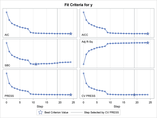
Output 44.2.13 shows how several fit statistics evolved as the selection process progressed. The five-fold CV PRESS statistic achieves its minimum at step 19. Note that this gives a larger model than was selected when the stopping criterion was determined using validation data. Furthermore, you see that the PRESS statistic has not achieved its minimum within 25 steps, so an even larger model would have been selected based on leave-one-out cross validation.
Output 44.2.14 shows how the average squared error compares on the test and training data. Note that the ASE error on the test data achieves a local minimum at step 11 and is already slowly increasing at step 19, which corresponds to the selected model.
The CVDETAILS=ALL option in the MODEL statement requests the "Cross Validation Details" table in Output 44.2.15 and the cross validation parameter estimates that are included in the "Parameter Estimates" table in Output 44.2.16. For each cross validation index, the predicted residual sum of squares on the observations omitted is shown in the "Cross Validation Details" table and the parameter estimates of the corresponding model are included in the "Parameter Estimates" table. By default, these details are shown for the selected model, but you can request this information at every step with the DETAILS= option in the MODEL statement. You use the "_CVINDEX_" variable in the output data set shown in Output 44.2.17 to find out which observations in the analysis data are omitted for each cross validation fold.
| Cross Validation Details | |||
|---|---|---|---|
| Index | Observations | CV PRESS | |
| Fitted | Left Out | ||
| 1 | 808 | 202 | 5059.7375 |
| 2 | 808 | 202 | 4278.9115 |
| 3 | 808 | 202 | 5598.0354 |
| 4 | 808 | 202 | 4950.1750 |
| 5 | 808 | 202 | 5528.1846 |
| Total | 25293.5024 | ||
| Parameter Estimates | |||||
|---|---|---|---|---|---|
| Parameter | Cross Validation Estimates | ||||
| 1 | 2 | 3 | 4 | 5 | |
| Intercept | 10.7617 | 10.1200 | 9.0254 | 13.4164 | 12.3352 |
| c1_3 | 28.2715 | 27.2977 | 27.0696 | 28.6835 | 27.8070 |
| c1_7 | 7.6530 | 7.6445 | 7.9257 | 7.4217 | 7.6862 |
| c3 tiny | -3.1103 | -4.4041 | -5.1793 | -8.4131 | -7.2096 |
| c3 small | 2.2039 | 1.5447 | 1.0121 | -0.3998 | 1.4927 |
| c3 average | 0.3021 | -1.3939 | -1.2201 | -3.3407 | -2.1467 |
| c3 big | -0.9621 | -1.2439 | -1.6092 | -3.7666 | -3.4389 |
| c3 huge | 0 | 0 | 0 | 0 | 0 |
| c1_3*c3 tiny | -21.9104 | -21.7840 | -22.0173 | -22.6066 | -21.9791 |
| c1_3*c3 small | -20.8196 | -20.2725 | -19.5850 | -20.4515 | -20.7586 |
| c1_3*c3 average | -16.8500 | -15.1509 | -15.0134 | -15.3851 | -13.4339 |
| c1_3*c3 big | -12.7212 | -12.1554 | -12.0354 | -12.3282 | -13.0174 |
| c1_3*c3 huge | 0 | 0 | 0 | 0 | 0 |
| x1 | 0.9238 | 1.7286 | 2.5976 | -0.2488 | 1.2093 |
| x1*c3 tiny | -1.5819 | -1.1748 | -3.2523 | -1.7016 | -2.7624 |
| x1*c3 small | -3.7669 | -3.2984 | -2.9755 | -1.8738 | -4.0167 |
| x1*c3 average | 2.2253 | 2.4489 | 1.5675 | 4.0948 | 2.0159 |
| x1*c3 big | 0.9222 | 0.5330 | 0.7960 | 2.6061 | 1.2694 |
| x1*c3 huge | 0 | 0 | 0 | 0 | 0 |
| x5 | -1.3562 | 0.5639 | 0.3022 | -0.4700 | -2.5063 |
| x6 | -0.9165 | -3.2944 | -1.2163 | -2.2063 | -0.5696 |
| x7 | 5.2295 | 5.3015 | 6.2526 | 4.1770 | 5.8364 |
| x6*x7 | 6.4211 | 7.5644 | 6.1182 | 7.0020 | 5.8730 |
| x10 | 1.9591 | 1.4932 | 0.7196 | 0.6504 | -0.3989 |
| x5*x10 | 3.6058 | 1.7274 | 4.3447 | 2.4388 | 3.8967 |
| x15 | -0.0079 | 0.6896 | 1.6811 | 0.0136 | 0.1799 |
| x15*c1_3 | -3.5022 | -2.7963 | -2.6003 | -4.2355 | -4.7546 |
| x7*x15 | -5.1438 | -5.8878 | -5.9465 | -3.6155 | -5.3337 |
| x18 | -2.1347 | -1.5656 | -2.4226 | -4.0592 | -1.4985 |
| x18*c3 tiny | 2.2988 | 1.1931 | 2.6491 | 6.1615 | 5.6204 |
| x18*c3 small | 4.6033 | 3.2359 | 4.4183 | 5.5923 | 1.7270 |
| x18*c3 average | -2.3712 | -2.5392 | -0.6361 | -1.1729 | -1.6481 |
| x18*c3 big | 2.3160 | 1.4654 | 2.7683 | 3.0487 | 2.5768 |
| x18*c3 huge | 0 | 0 | 0 | 0 | 0 |
| x6*x18 | 3.0716 | 4.2036 | 4.1354 | 4.9196 | 2.7165 |
| x20 | 4.1229 | 4.5773 | 4.5774 | 4.6555 | 4.2655 |
The following statements display the first eight observations in the outData data set.
proc print data=outData(obs=8);
run;
| Obs | c3 | x1 | x2 | x3 | x4 | x5 | x6 | x7 | x8 | x9 | x10 | x11 | x12 | x13 | x14 | x15 | x16 | x17 | x18 | x19 | x20 | c1 | c2 | y | _CVINDEX_ | p_y |
|---|---|---|---|---|---|---|---|---|---|---|---|---|---|---|---|---|---|---|---|---|---|---|---|---|---|---|
| 1 | tiny | 0.18496 | 0.97009 | 0.39982 | 0.25940 | 0.92160 | 0.96928 | 0.54298 | 0.53169 | 0.04979 | 0.06657 | 0.81932 | 0.52387 | 0.85339 | 0.06718 | 0.95702 | 0.29719 | 0.27261 | 0.68993 | 0.97676 | 0.22651 | 2 | 1 | 11.4391 | 1 | 18.1474 |
| 2 | tiny | 0.47579 | 0.84499 | 0.63452 | 0.59036 | 0.58258 | 0.37701 | 0.72836 | 0.50660 | 0.93121 | 0.92912 | 0.58966 | 0.29722 | 0.39104 | 0.47243 | 0.67953 | 0.16809 | 0.16653 | 0.87110 | 0.29879 | 0.93464 | 3 | 1 | 31.4596 | 2 | 24.7930 |
| 3 | tiny | 0.51132 | 0.43320 | 0.17611 | 0.66504 | 0.40482 | 0.12455 | 0.45349 | 0.19955 | 0.57484 | 0.73847 | 0.43981 | 0.04937 | 0.52238 | 0.34337 | 0.02271 | 0.71289 | 0.93706 | 0.44599 | 0.94694 | 0.71290 | 4 | 3 | 16.4294 | 3 | 16.5752 |
| 4 | tiny | 0.42071 | 0.07174 | 0.35849 | 0.71143 | 0.18985 | 0.14797 | 0.56184 | 0.27011 | 0.32520 | 0.56918 | 0.04259 | 0.43921 | 0.91744 | 0.52584 | 0.73182 | 0.90522 | 0.57600 | 0.18794 | 0.33133 | 0.69887 | 5 | 3 | 15.4815 | 4 | 14.7605 |
| 5 | tiny | 0.42137 | 0.03798 | 0.27081 | 0.42773 | 0.82010 | 0.84345 | 0.87691 | 0.26722 | 0.30602 | 0.39705 | 0.34905 | 0.76593 | 0.54340 | 0.61257 | 0.55291 | 0.73591 | 0.37186 | 0.64565 | 0.55718 | 0.87504 | 6 | 2 | 26.0023 | 5 | 24.7479 |
| 6 | tiny | 0.81722 | 0.65822 | 0.02947 | 0.85339 | 0.36285 | 0.37732 | 0.51054 | 0.71194 | 0.37533 | 0.22954 | 0.68621 | 0.55243 | 0.58182 | 0.17472 | 0.04610 | 0.64380 | 0.64545 | 0.09317 | 0.62008 | 0.07845 | 7 | 1 | 16.6503 | 1 | 21.4444 |
| 7 | tiny | 0.19480 | 0.81673 | 0.08548 | 0.18376 | 0.33264 | 0.70558 | 0.92761 | 0.29642 | 0.22404 | 0.14719 | 0.59064 | 0.46326 | 0.41860 | 0.25631 | 0.23045 | 0.08034 | 0.43559 | 0.67020 | 0.42272 | 0.49827 | 1 | 1 | 14.0342 | 2 | 20.9661 |
| 8 | tiny | 0.04403 | 0.51697 | 0.68884 | 0.45333 | 0.83565 | 0.29745 | 0.40325 | 0.95684 | 0.42194 | 0.78079 | 0.33106 | 0.17210 | 0.91056 | 0.26897 | 0.95602 | 0.13720 | 0.27190 | 0.55692 | 0.65825 | 0.68465 | 2 | 3 | 14.9830 | 3 | 17.5644 |
This example demonstrates the usefulness of effect selection when you suspect that interactions of effects are needed to explain the variation in your dependent variable. Ideally, a priori knowledge should be used to decide what interactions to allow, but in some cases this information might not be available. Simply fitting a least squares model allowing all interactions produces a model that overfits your data and generalizes very poorly.
The following statements use forward selection with selection based on the SBC criterion, which is the default selection criterion. At each step, the effect whose addition to the model yields the smallest SBC value is added. The STOP=NONE suboption specifies that this process continue even when the SBC statistic grows whenever an effect is added, and so it terminates at a full least squares model. The BUILDSSCP=FULL option is specified in a PERFORMANCE statement, since building the SSCP matrix incrementally is counterproductive in this case. See the section for details. Note that if all you are interested in is a full least squares model, then it is much more efficient to simply specify SELECTION=NONE in the MODEL statement. However, in this example the aim is to add effects in roughly increasing order of explanatory power.
proc glmselect data=analysisData testdata=testData plots=ASEPlot;
   class c1 c2 c3(order=data);
   model y =  c1|c2|c3|x1|x2|x3|x4|x5|x5|x6|x7|x8|x9|x10
             |x11|x12|x13|x14|x15|x16|x17|x18|x19|x20 @2
           / selection=forward(stop=none)
             hierarchy=single;
   performance buildSSCP = full;
run;

ods graphics off;
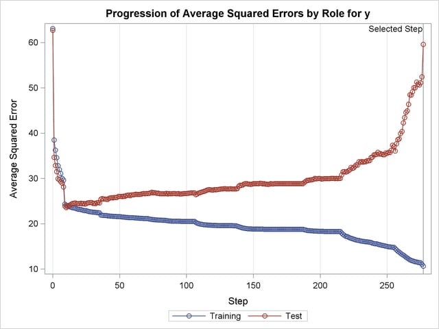
The ASE plot shown in Output 44.2.18 clearly demonstrates the danger in overfitting the training data. As more insignificant effects are added to the model, the growth in test set ASE shows how the predictions produced by the resulting models worsen. This decline is particularly rapid in the latter stages of the forward selection, because the use of the SBC criterion results in insignificant effects with lots of parameters being added after insignificant effects with fewer parameters.