The GLMSELECT Procedure
-
Overview

- Getting Started
-
Syntax
-
Details
Model-Selection Methods Model Selection Issues Criteria Used in Model Selection Methods CLASS Variable Parameterization and the SPLIT Option Macro Variables Containing Selected Models Using the STORE Statement Building the SSCP Matrix Model Averaging Using Validation and Test Data Cross Validation Displayed Output ODS Table Names ODS Graphics
-
Examples
- References
Example 44.1 Modeling Baseball Salaries Using Performance Statistics
This example continues the investigation of the baseball data set introduced in the section Getting Started: GLMSELECT Procedure. In that example, the default stepwise selection method based on the SBC criterion was used to select a model. In this example, model selection that uses other information criteria and out-of-sample prediction criteria is explored.
PROC GLMSELECT provides several selection algorithms that you can customize by specifying criteria for selecting effects, stopping the selection process, and choosing a model from the sequence of models at each step. For more details on the criteria available, see the section Criteria Used in Model Selection Methods. The SELECT=SL suboption of the SELECTION= option in the MODEL statement in the following code requests the traditional hypothesis test-based stepwise selection approach, where effects in the model that are not significant at the stay significance level (SLS) are candidates for removal and effects not yet in the model whose addition is significant at the entry significance level (SLE) are candidates for addition to the model.
ods graphics on;

proc glmselect data=baseball plot=CriterionPanel;
  class league division;
  model logSalary = nAtBat nHits nHome nRuns nRBI nBB
                 yrMajor crAtBat crHits crHome crRuns crRbi
                 crBB league division nOuts nAssts nError
               / selection=stepwise(select=SL) stats=all;
run;
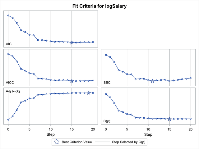
The default SLE and SLS values of 0.15 might not be appropriate for these data. One way to investigate alternative ways to stop the selection process is to assess the sequence of models in terms of model fit statistics. The STATS=ALL option in the MODEL statement requests that all model fit statistics for assessing the sequence of models of the selection process be displayed. To help in the interpretation of the selection process, you can use graphics supported by PROC GLMSELECT. ODS Graphics must be enabled before requesting plots. For general information about ODS Graphics, see Chapter 21, Statistical Graphics Using ODS. With ODS Graphics enabled, the PLOTS=CRITRERIONPANEL option in the PROC GLMSELECT statement produces the criterion panel shown in Output 44.1.1.
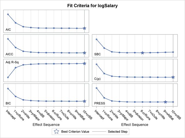
You can see in Output 44.1.1 that this stepwise selection process would stop at an earlier step if you use the Schwarz Bayesian information criterion (SBC) or predicted residual sum of squares (PRESS) to assess the selected models as stepwise selection progresses. You can use the CHOOSE= suboption of the SELECTION= option in the MODEL statement to specify the criterion you want to use to select among the evaluated models. The following statements use the PRESS statistic to choose among the models evaluated during the stepwise selection.
proc glmselect data=baseball;
  class league division;
  model logSalary = nAtBat nHits nHome nRuns nRBI nBB
                 yrMajor crAtBat crHits crHome crRuns crRbi
                 crBB league division nOuts nAssts nError
               / selection=stepwise(select=SL choose=PRESS);
run;
Note that the selected model is the model at step 9. By default, PROC GLMSELECT displays the selected model, ANOVA and fit statistics, and parameter estimates for the selected model. These are shown in Output 44.1.2.
| Effects: | Intercept nAtBat nHits nBB yrMajor crHits division nOuts |
|---|
| Analysis of Variance | ||||
|---|---|---|---|---|
| Source | DF | Sum of Squares |
Mean Square |
F Value |
| Model | 7 | 124.67715 | 17.81102 | 55.07 |
| Error | 255 | 82.47658 | 0.32344 | |
| Corrected Total | 262 | 207.15373 | ||
| Root MSE | 0.56872 |
|---|---|
| Dependent Mean | 5.92722 |
| R-Square | 0.6019 |
| Adj R-Sq | 0.5909 |
| AIC | -23.98522 |
| AICC | -23.27376 |
| PRESS | 88.55275 |
| SBC | -260.40799 |
| Parameter Estimates | ||||
|---|---|---|---|---|
| Parameter | DF | Estimate | Standard Error | t Value |
| Intercept | 1 | 4.176133 | 0.150539 | 27.74 |
| nAtBat | 1 | -0.001468 | 0.000946 | -1.55 |
| nHits | 1 | 0.011078 | 0.002983 | 3.71 |
| nBB | 1 | 0.007226 | 0.002115 | 3.42 |
| yrMajor | 1 | 0.070056 | 0.018911 | 3.70 |
| crHits | 1 | 0.000247 | 0.000143 | 1.72 |
| division East | 1 | 0.143082 | 0.070972 | 2.02 |
| division West | 0 | 0 | . | . |
| nOuts | 1 | 0.000241 | 0.000134 | 1.81 |
Even though the model that is chosen to give the smallest value of the PRESS statistic is the model at step 9, the stepwise selection process continues to the step where the stopping condition based on entry and stay significance levels is met. If you use the PRESS statistic as the stopping criterion, the stepwise selection process stops at step 9. This ability to stop at the first extremum of the criterion you specify can significantly reduce the amount of computation done, especially in the cases where you are selecting from a large number of effects. The following statements request stopping based on the PRESS statistic. The stop reason and stop details tables are shown in Output 44.1.3.
proc glmselect data=baseball plot=Coefficients;
  class league division;
  model logSalary = nAtBat nHits nHome nRuns nRBI nBB
                 yrMajor crAtBat crHits crHome crRuns crRbi
                 crBB league division nOuts nAssts nError
               / selection=stepwise(select=SL stop=PRESS);
run;
| Selection stopped at a local minimum of the PRESS criterion. |
| Stop Details | ||||
|---|---|---|---|---|
| Candidate For |
Effect | Candidate PRESS |
Compare PRESS |
|
| Entry | crBB | 88.6321 | > | 88.5528 |
| Removal | nAtBat | 88.6866 | > | 88.5528 |
The PLOTS=COEFFICIENTS specification in the PROC GLMSELECT statement requests a plot that enables you to visualize the selection process.
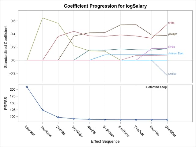
Output 44.1.4 shows the standardized coefficients of all the effects selected at some step of the stepwise method plotted as a function of the step number. This enables you to assess the relative importance of the effects selected at any step of the selection process as well as providing information as to when effects entered the model. The lower plot in the panel shows how the criterion used to choose the selected model changes as effects enter or leave the model.
Model selection is often done in order to obtain a parsimonious model that can be used for prediction on new data. An ever-present danger is that of selecting a model that overfits the "training" data used in the fitting process, yielding a model with poor predictive performance. Using cross validation is one way to assess the predictive performance of the model. Using  -fold cross validation, the training data are subdivided into parts, and at each step of the selection process, models are obtained on each of the subsets of the data obtained by omitting one of these parts. The cross validation predicted residual sum of squares, denoted CV PRESS, is obtained by summing the squares of the residuals when each of these submodels is scored on the data omitted in fitting the submodel. Note that the PRESS statistic corresponds to the special case of "leave-one-out" cross validation.
In the preceding example, the PRESS statistic was used to choose among models that were chosen based on entry and stay significance levels. In the following statements, the SELECT=CVPRESS suboption of the SELECTION= option in the MODEL statement requests that the CV PRESS statistic itself be used as the selection criterion. The DROP=COMPETITIVE suboption requests that additions and deletions be considered simultaneously when deciding whether to add or remove an effect. At any step, the CV PRESS statistic for all models obtained by deleting one effect from the model or adding one effect to the model is computed. Among these models, the one yielding the smallest value of the CV PRESS statistic is selected and the process is repeated from this model. The stepwise selection terminates if all additions or deletions increase the CV PRESS statistic. The CVMETHOD=SPLIT(5) option requests five-fold cross validation with the five subsets consisting of observations  ,
,  , and so on.
proc glmselect data=baseball plot=Candidates;
  class league division;
  model logSalary = nAtBat nHits nHome nRuns nRBI nBB
                 yrMajor crAtBat crHits crHome crRuns crRbi
                 crBB league division nOuts nAssts nError
               / selection=stepwise(select=CV drop=competitive)
                 cvMethod=split(5);
run;
The selection summary table is shown in Output 44.1.5. By comparing Output 44.1.5 and Output 44.6 you can see that the sequence of models produced is different from the sequence when the stepwise selection is based on the SBC statistic.
| Stepwise Selection Summary | |||||
|---|---|---|---|---|---|
| Step | Effect Entered |
Effect Removed |
Number Effects In |
Number Parms In |
CV PRESS |
| 0 | Intercept | 1 | 1 | 208.9638 | |
| 1 | crRuns | 2 | 2 | 122.5755 | |
| 2 | nHits | 3 | 3 | 96.3949 | |
| 3 | yrMajor | 4 | 4 | 92.2117 | |
| 4 | nBB | 5 | 5 | 89.5242 | |
| 5 | crRuns | 4 | 4 | 88.6917 | |
| 6 | league | 5 | 5 | 88.0417 | |
| 7 | nError | 6 | 6 | 87.3170 | |
| 8 | division | 7 | 7 | 87.2147 | |
| 9 | nHome | 8 | 8 | 87.0960* | |
| * Optimal Value Of Criterion | |||||
If you have sufficient data, another way you can assess the predictive performance of your model is to reserve part of your data for testing your model. You score the model obtained using the training data on the test data and assess the predictive performance on these data that had no role in the selection process. You can also reserve part of your data to validate the model you obtain in the training process. Note that the validation data are not used in obtaining the coefficients of the model, but they are used to decide when to stop the selection process to limit overfitting.
PROC GLMSELECT enables you to partition your data into disjoint subsets for training validation and testing roles. This partitioning can be done by using random proportions of the data, or you can designate a variable in your data set that defines which observations to use for each role. See the section PARTITION Statement for more details.
The following statements randomly partition the baseball data set, using 50% for training, 30% for validation, and 20% for testing. The model selected at each step is scored on the validation data, and the average residual sums of squares (ASE) is evaluated. The model yielding the lowest ASE on the validation data is selected. The ASE on the test data is also evaluated, but these data play no role in the selection process. Note that a seed for the pseudo-random number generator is specified in the PROC GLMSELECT statement.
proc glmselect data=baseball plots=(CriterionPanel ASE) seed=1;
  partition fraction(validate=0.3 test=0.2);
  class league division;
  model logSalary = nAtBat nHits nHome nRuns nRBI nBB
                 yrMajor crAtBat crHits crHome crRuns crRbi
                 crBB league division nOuts nAssts nError
               / selection=forward(choose=validate stop=10);
run;
| Number of Observations Read | 322 |
|---|---|
| Number of Observations Used | 263 |
| Number of Observations Used for Training | 132 |
| Number of Observations Used for Validation | 80 |
| Number of Observations Used for Testing | 51 |
Output 44.1.6 shows the number of observation table. You can see that of the 263 observations that were used in the analysis, 132 (50.2%) observations were used for model training, 80 (30.4%) for model validation, and 51 (19.4%) for model testing.
| Forward Selection Summary | |||||||
|---|---|---|---|---|---|---|---|
| Step | Effect Entered |
Number Effects In |
Number Parms In |
SBC | ASE | Validation ASE |
Test ASE |
| 0 | Intercept | 1 | 1 | -30.8531 | 0.7628 | 0.7843 | 0.8818 |
| 1 | crRuns | 2 | 2 | -93.9367 | 0.4558 | 0.4947 | 0.4210 |
| 2 | nHits | 3 | 3 | -126.2647 | 0.3439 | 0.3248 | 0.4697 |
| 3 | yrMajor | 4 | 4 | -128.7570 | 0.3252 | 0.2920* | 0.4614 |
| 4 | nBB | 5 | 5 | -132.2409* | 0.3052 | 0.3065 | 0.4297 |
| 5 | division | 6 | 6 | -130.7794 | 0.2974 | 0.3050 | 0.4218 |
| 6 | nOuts | 7 | 7 | -128.5897 | 0.2914 | 0.3028 | 0.4186 |
| 7 | nRBI | 8 | 8 | -125.7825 | 0.2868 | 0.3097 | 0.4489 |
| 8 | nHome | 9 | 9 | -124.7709 | 0.2786 | 0.3383 | 0.4533 |
| 9 | nAtBat | 10 | 10 | -121.3767 | 0.2754 | 0.3337 | 0.4580 |
| * Optimal Value Of Criterion | |||||||
| Selection stopped at the first model containing the specified number of effects (10). |
Output 44.1.7 shows the selection summary table and the stop reason. The forward selection stops at step 9 since the model at this step contains 10 effects, and so it satisfies the stopping criterion requested with the "STOP=10" suboption. However, the selected model is the model at step 3, where the validation ASE, the CHOOSE= criterion, achieves its minimum.
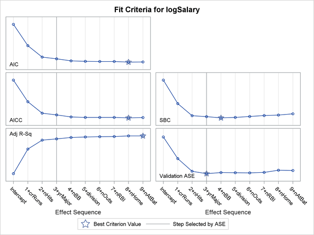
The criterion panel in Output 44.1.8 shows how the various criteria evolved as the stepwise selection method proceeded. Note that other than the ASE evaluated on the validation data, these criteria are evaluated on the training data.
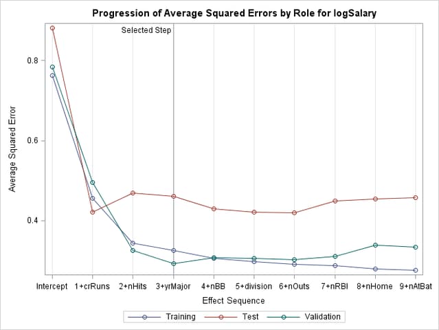
Finally, the ASE plot in Output 44.1.9 shows how the average square error evolves on the training, validation, and test data. Note that while the ASE on the training data continued decreasing as the selection steps proceeded, the ASE on the test and validation data behave more erratically.
LASSO selection, pioneered by Tibshirani (1996), is a constrained least squares method that can be viewed as a stepwise-like method where effects enter and leave the model sequentially. You can find additional details about the LASSO method in the section Lasso Selection (LASSO). Note that when classification effects are used with LASSO, the design matrix columns for all effects containing classification variables can enter or leave the model individually. The following statements perform LASSO selection for the baseball data. The LASSO selection summary table is shown in Output 44.1.10.
 proc glmselect data=baseball plot=CriterionPanel ;
  class league division;
  model logSalary = nAtBat nHits nHome nRuns nRBI nBB
                 yrMajor crAtBat crHits crHome crRuns crRbi
                 crBB league division nOuts nAssts nError
               / selection=lasso(choose=CP steps=20);
run;

ods graphics off;
| LASSO Selection Summary | ||||
|---|---|---|---|---|
| Step | Effect Entered |
Effect Removed |
Number Effects In |
CP |
| 0 | Intercept | 1 | 375.9275 | |
| 1 | crRuns | 2 | 328.6492 | |
| 2 | crHits | 3 | 239.5392 | |
| 3 | nHits | 4 | 134.0374 | |
| 4 | nBB | 5 | 111.6638 | |
| 5 | crRbi | 6 | 81.7296 | |
| 6 | yrMajor | 7 | 75.0428 | |
| 7 | nRBI | 8 | 30.4494 | |
| 8 | division_East | 9 | 29.9913 | |
| 9 | nOuts | 10 | 25.1656 | |
| 10 | crRuns | 9 | 18.7295 | |
| 11 | crRbi | 8 | 15.1683 | |
| 12 | nError | 9 | 16.6233 | |
| 13 | nHome | 10 | 16.3741 | |
| 14 | league_American | 11 | 14.8794 | |
| 15 | nRBI | 10 | 8.8477* | |
| 16 | crBB | 11 | 9.2242 | |
| 17 | crRuns | 12 | 10.7608 | |
| 18 | nAtBat | 13 | 11.6266 | |
| 19 | nAssts | 14 | 11.8572 | |
| 20 | crAtBat | 15 | 13.4020 | |
| * Optimal Value Of Criterion | ||||
| Selection stopped at the specified number of steps (20). |
Note that effects enter and leave sequentially. In this example, the STEPS= suboption of the SELECTION= option specifies that 20 steps of LASSO selection be done. You can see how the various model fit statistics evolved in Output 44.1.11.
The CHOOSE=CP suboption specifies that the selected model be the model at step 15 that yields the optimal value of Mallows’ C( ) statistic. Details of this selected model are shown in Output 44.1.12.
| Effects: | Intercept nHits nHome nBB yrMajor crHits league_American division_East nOuts nError |
|---|
| Analysis of Variance | ||||
|---|---|---|---|---|
| Source | DF | Sum of Squares |
Mean Square |
F Value |
| Model | 9 | 125.24302 | 13.91589 | 42.98 |
| Error | 253 | 81.91071 | 0.32376 | |
| Corrected Total | 262 | 207.15373 | ||
| Root MSE | 0.56900 |
|---|---|
| Dependent Mean | 5.92722 |
| R-Square | 0.6046 |
| Adj R-Sq | 0.5905 |
| AIC | -21.79589 |
| AICC | -20.74409 |
| BIC | -283.91417 |
| C(p) | 8.84767 |
| SBC | -251.07435 |
| Parameter Estimates | ||
|---|---|---|
| Parameter | DF | Estimate |
| Intercept | 1 | 4.204236 |
| nHits | 1 | 0.006942 |
| nHome | 1 | 0.002785 |
| nBB | 1 | 0.005727 |
| yrMajor | 1 | 0.067054 |
| crHits | 1 | 0.000249 |
| league_American | 1 | -0.079607 |
| division_East | 1 | 0.134723 |
| nOuts | 1 | 0.000183 |
| nError | 1 | -0.007213 |