The GLMSELECT Procedure

ODS Graph Names

PROC GLMSELECT assigns a name to each graph it creates using ODS. You can use these names to reference the graphs when using ODS. The names are listed in Table 44.9.

Candidates Plot

You request the "Candidates Plot" by specifying the PLOTS=CANDIDATES option in the PROC GLMSELECT statement and the DETAILS=STEPS option in the MODEL statement. This plot shows the values of selection criterion for the candidate effects for entry or removal, sorted from best to worst from left to right across the plot. The leftmost candidate displayed is the effect selected for entry or removal at that step. You can use this plot to see at what steps the decision about which effect to add or drop is clear-cut. See Figure 44.5 for an example.

Coefficient Panel

When you specify the PLOTS=COEFFICIENTS option in the PROC GLMSELECT statement, PROC GLMSELECT produces a panel of two plots showing how the standardized coefficients and the criterion used to choose the final model evolve as the selection progresses. The following statements provide an example:

ods graphics on;

proc glmselect data=baseball plots=coefficients;
  class league division; 
  model logSalary = nAtBat nHits nHome nRuns nRBI nBB
                    yrMajor|yrMajor crAtBat|crAtBat crHits|crHits
                    crHome|crHome crRuns|crRuns crRbi|crRbi  
                    crBB|crBB league division nOuts nAssts nError /
                    selection=forward(stop=AICC CHOOSE=SBC);
run;   

Figure 44.16 shows the requested graphic. The upper plot in the panel displays the standardized coefficients as a function of the step number. You can request standardized coefficients in the parameter estimates tables by specifying the STB option in the MODEL statement, but this option is not required to produce this plot. To help in tracing the changes in a parameter, the standardized coefficients for each parameter are connected by lines. Coefficients corresponding to effects that are not in the selected model at a step are zero and hence not observable. For example, consider the parameter crAtBat*crAtBat in Output 44.16. Because crAtBat*crAtBat enters the model at step 2, the line that represents this parameter starts rising from zero at step 1 when crRuns enters the model. Parameters that are nonzero at the final step of the selection are labeled if their magnitudes are greater than 1% of the range of the magnitudes of all the nonzero parameters at this step. To avoid collision, labels corresponding to parameters with similar values at the final step might get suppressed. You can control when this label collision avoidance occurs by using the LABELGAP= suboption of the PLOTS=COEFFICIENTS option. Planned enhancements to the automatic label collision avoidance algorithm will obviate the need for this option in future releases of the GLMSELECT procedure.

Figure 44.16 Coefficient Panel

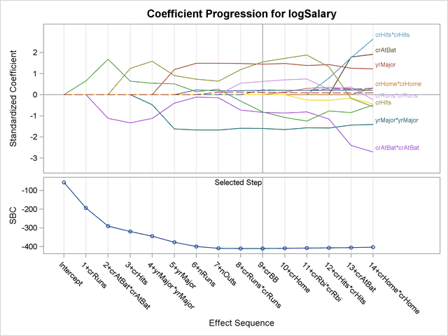
The lower plot in the panel shows how the criterion used to choose among the examined models progresses. The selected step occurs at the optimal value of this criterion. In this example, this criterion is the SBC criterion and it achieves its minimal value at step 9 of the forward selection.

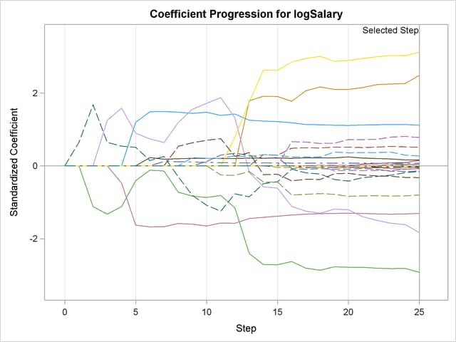
In some cases, particularly when the final step contains a large number of parameters, you might be interested in using this plot only to discern if and when the parameters in the model are essential unchanged beyond a certain step. In such cases, you might want to suppress the labeling of the parameters and use a numeric axis on the horizontal axis of the plot. You can do this using the STEPAXIS= and MAXPARMLABEL= suboptions of the PLOTS=CRITERIA option. The following statements provide an example:

proc glmselect data=baseball 
     plots(unpack maxparmlabel=0 stepaxis=number)=coefficients;

  class league division; 
  model logSalary = nAtBat nHits nHome nRuns nRBI nBB
                    yrMajor|yrMajor crAtBat|crAtBat crHits|crHits
                    crHome|crHome crRuns|crRuns crRbi|crRbi  
                    crBB|crBB league division nOuts nAssts nError /
                    selection=forward(stop=none);
run;  

The UNPACK = option requests that the plots of the coefficients and CHOOSE= criterion be shown in separate plots. The STEPAXIS=NUMBER option requests a numeric horizontal axis showing step number, and the MAXPAMLABEL=0 option suppresses the labels for the parameters. The "Coefficient Plot" is shown in Figure 44.17. You can see that the standardized coefficients do not vary greatly after step 16.

Figure 44.17 Coefficient Plot

Criterion Panel

You request the criterion panel by specifying the PLOTS=CRITERIA option in the PROC GLMSELECT statement. This panel displays the progression of the ADJRSQ, AIC, AICC, and SBC criteria, as well as any other criteria that are named in the CHOOSE=, SELECT=, STOP=, or STATS= option in the MODEL statement.

The following statements provide an example:

proc glmselect data=baseball plots=criteria;
  class league division; 
  model logSalary = nAtBat nHits nHome nRuns nRBI nBB
                    yrMajor|yrMajor crAtBat|crAtBat crHits|crHits
                    crHome|crHome crRuns|crRuns crRbi|crRbi  
                    crBB|crBB league division nOuts nAssts nError /
                    selection=forward(steps=15 choose=AICC)
                    stats=PRESS;
run;  

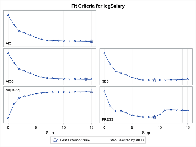
Figure 44.18 shows the requested criterion panel. Note that the PRESS criterion is included in the panel because it is named in the STATS= option in the MODEL statement. The selected step is displayed as a vertical reference line on the plot of each criterion, and the legend indicates which of these criteria is used to make the selection. If the selection terminates for a reason other than optimizing a criterion displayed on this plot, then the legend will not report a reason for the selected step. The optimal value of each criterion is indicated with the "Star" marker. Note that it is possible that a better value of a criterion might have been reached had more steps of the selection process been done.

Figure 44.18 Criterion Panel

Average Square Error Plot

You request the average square error plot by specifying the PLOTS=ASE option in the PROC GLMSELECT statement. This plot shows the progression of the average square error (ASE) evaluated separately on the training data, and the test and validation data whenever these data are provided with the TESTDATA= and VALDATA= options or are produced by using a PARTITION statement. You use the plot to detect when overfitting the training data occurs. The ASE decreases monotonically on the training data as parameters are added to a model. However, the average square error on test and validation data typically starts increasing when overfitting occurs. See Output 44.1.9 and Output 44.2.6 for examples.

Examining Specific Step Ranges

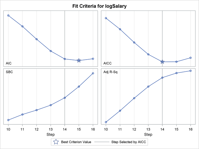
The coefficient panel, criterion panel, and average square error plot display information for all the steps examined in the selection process. In some cases, you might want to focus attention on just a particular step range. For example, it is hard to discern the variation in the criteria displayed in Figure 44.18 near the selected step because the variation in these criteria in the steps close to the selected step is small relative to the variation across all steps. You can request a range of steps to display using the STARTSTEP= and ENDSTEP= suboptions of the PLOTS= option. You can specify these options as both global and specific plot options, with the specific options taking precedence if both are specified. The following statements provide an example:

proc glmselect data=baseball plots=criteria(startstep=10 endstep=16);
  class league division; 
  model logSalary = nAtBat nHits nHome nRuns nRBI nBB
                    yrMajor|yrMajor crAtBat|crAtBat crHits|crHits
                    crHome|crHome crRuns|crRuns crRbi|crRbi  
                    crBB|crBB league division nOuts nAssts nError /
                    selection=forward(stop=none choose=AICC);
run;  

ods graphics off;

Figure 44.19 shows the progression of the fit criteria between steps 10 and 16. Note that if the optimal value of a criterion does not occur in this specified step range, then no optimal marker appears for that criterion. The plot of the SBC criterion in Figure 44.19 is one such case.

Figure 44.19 Criterion Panel for Specified Step Range