The GLMSELECT Procedure

As discussed in the section Model Selection Issues, some well-known issues arise in performing model selection for inference and prediction. One approach to address these issues is to use resampled data as a proxy for multiple samples that are drawn from some conceptual probability distribution. A model is selected for each resampled set of data, and a predictive model is built by averaging the predictions of these selected models. You can perform this method of model averaging by using the MODELAVERAGE statement. Resampling-based methods, in which samples are obtained by drawing with replacement from your data, fall under the umbrella of the widely studied methodology known as the bootstrap (Efron and Tibshirani, 1993). For use of the bootstrap in the context of variable selection, see Breiman(1992).

By default, when the average is formed, models that are selected in multiple samples receive more weight than infrequently selected models. Alternatively, you can start by fitting a prespecified set of models on your data, then use information-theoretic approaches to assign a weight to each model in building a weighted average model. You can find a detailed discussion of this methodology in Burnham and Anderson (2002), in addition to some comparisons of this approach with bootstrap-based methods.

In the linear model context, the average prediction that you obtain from a set of models is the same as the prediction that you obtain with the single model whose parameter estimates are the averages of the corresponding estimates of the set of models. Hence, you can regard model averaging as a selection method that selects this average model. To show this, denote by the parameter estimates for the sample where if parameter is not in the selected model for sample . Then the predicted values for average model are given by

where is the design matrix of the data to be scored. Forming averages gives

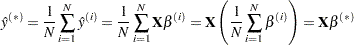where for parameter , .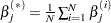

You can see that if a parameter estimate is nonzero for just a few of the sample models, then averaging the estimates for this parameter shrinks this estimate towards zero. It is this shrinkage that ameliorates the bias that a parameter is more likely to be selected if it is above its expected value rather than below it. This reduction in bias often produces improved predictions on new data that you obtain with the average model. However, the average model is not parsimonious since it has nonzero estimates for any parameter that is selected in any sample.

One resampling-based approach for obtaining a parsimonious model is to use the number of times that regressors are selected as an indication of importance and then to fit a new model that uses just the regressors that you deem to be most important. This approach is not without risk. One possible problem is that you might have several regressors that, for purposes of prediction, can be used as surrogates for one another. In this case it is possible that none of these regressors individually appears in a large enough percentage of the sample models to be deemed important, even though every model contains at least one of them. Despite such potential problems, this strategy is often successful. You can implement this approach by using the REFIT option in the MODELAVERAGE statement. By default, the REFIT option performs a second round of model averaging, where a fixed model that consists of the effects that are selected in a least twenty percent of the samples in the initial round of model averaging is used. The average model is obtained by averaging the ordinary least squares estimates obtained for each sample in the refit. Note that the default selection frequency cutoff of twenty percent is merely a heuristic guideline that often produces reasonable models.

Another approach to obtaining a parsimonious average model is to form the average of just the frequently selected models. You can implement this strategy by using the SUBSET option in the MODELAVERAGE statement. However, in situations where there are many irrelevant regressors, it is often the case that most of the selected models are selected just once. In such situations, having a way to order the models that are selected with the same frequency is desirable. The following section discusses a way to do this.

Model Selection Frequencies and Frequency Scores

The model frequency score orders models by their selection frequency, but also uses effect selection frequencies to order different models that are selected with the same frequency. Let denote the th effect and let denote the selection fraction for this effect. is computed as the number of samples whose selected model contains effect divided by the number of samples. Suppose the th model that consists of the effects is selected times. Then the model frequency score, , for this model is computed as the sum of the model selection frequency and the average selection fraction for this model; that is,

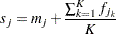When you use the BEST= suboption of the SUBSET option in the MODELAVERAGE statement, then the average model is formed from the models with the largest model frequency scores.