The UNIVARIATE Procedure

Example 4.25 Annotating a Folded Normal Curve

This example shows how to display a fitted curve that is not supported by the HISTOGRAM statement. The offset of an attachment point is measured (in mm) for a number of manufactured assemblies, and the measurements (Offset) are saved in a data set named Assembly. The following statements create the data set Assembly:

data Assembly;
   label Offset = 'Offset (in mm)';
   input Offset @@;
   datalines;
11.11 13.07 11.42  3.92 11.08  5.40 11.22 14.69  6.27  9.76
 9.18  5.07  3.51 16.65 14.10  9.69 16.61  5.67  2.89  8.13
 9.97  3.28 13.03 13.78  3.13  9.53  4.58  7.94 13.51 11.43
11.98  3.90  7.67  4.32 12.69  6.17 11.48  2.82 20.42  1.01
 3.18  6.02  6.63  1.72  2.42 11.32 16.49  1.22  9.13  3.34
 1.29  1.70  0.65  2.62  2.04 11.08 18.85 11.94  8.34  2.07
 0.31  8.91 13.62 14.94  4.83 16.84  7.09  3.37  0.49 15.19
 5.16  4.14  1.92 12.70  1.97  2.10  9.38  3.18  4.18  7.22
15.84 10.85  2.35  1.93  9.19  1.39 11.40 12.20 16.07  9.23
 0.05  2.15  1.95  4.39  0.48 10.16  4.81  8.28  5.68 22.81
 0.23  0.38 12.71  0.06 10.11 18.38  5.53  9.36  9.32  3.63
12.93 10.39  2.05 15.49  8.12  9.52  7.77 10.70  6.37  1.91
 8.60 22.22  1.74  5.84 12.90 13.06  5.08  2.09  6.41  1.40
15.60  2.36  3.97  6.17  0.62  8.56  9.36 10.19  7.16  2.37
12.91  0.95  0.89  3.82  7.86  5.33 12.92  2.64  7.92 14.06
;

It is decided to fit a folded normal distribution to the offset measurements. A variable $\text{[math]}$ has a folded normal distribution if $\text{[math]}$ , where $\text{[math]}$ is distributed as $\text{[math]}$ . The fitted density is

$\text{[math]}$

where $\text{[math]}$ .

You can use SAS/IML to compute preliminary estimates of $\text{[math]}$ and $\text{[math]}$ based on a method of moments given by Elandt (1961). These estimates are computed by solving equation (19) Elandt (1961), which is given by

$\text{[math]}$

where $\text{[math]}$ is the standard normal distribution function and

$\text{[math]}$

Then the estimates of $\text{[math]}$ and $\text{[math]}$ are given by

$\text{[math]}$

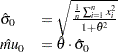Begin by using PROC MEANS to compute the first and second moments and by using the following DATA step to compute the constant $\text{[math]}$ :

proc means data = Assembly noprint;
   var Offset;
   output out=stat mean=m1 var=var n=n min = min;
run;

* Compute constant A from equation (19) of Elandt (1961);
data stat;
   keep m2 a min;
   set stat;
   a  = (m1*m1);
   m2 = ((n-1)/n)*var + a;
   a  = a/m2;
run;

Next, use the SAS/IML subroutine NLPDD to solve equation (19) by minimizing $\text{[math]}$ , and compute $\text{[math]}$ and $\text{[math]}$ :

proc iml;
   use stat;
   read all var {m2}  into m2;
   read all var {a}   into a;
   read all var {min} into min;

   * f(t) is the function in equation (19) of Elandt (1961);
   start f(t) global(a);
     y = .39894*exp(-0.5*t*t);
     y = (2*y-(t*(1-2*probnorm(t))))**2/(1+t*t);
     y = (y-a)**2;
     return(y);
   finish;

   * Minimize (f(t)-A)**2 and estimate mu and sigma;
   if ( min < 0 ) then do;
      print "Warning: Observations are not all nonnegative.";
      print "     The folded normal is inappropriate.";
      stop;
      end;
   if ( a < 0.637 ) then do;
      print "Warning: the folded normal may be inappropriate";
      end;
   opt = { 0 0 };
   con = { 1e-6 };
   x0  = { 2.0 };
   tc  = { . . . . . 1e-8 . . . . . . .};
   call nlpdd(rc,etheta0,"f",x0,opt,con,tc);
   esig0 = sqrt(m2/(1+etheta0*etheta0));
   emu0  = etheta0*esig0;

   create prelim var {emu0 esig0 etheta0};
   append;
   close prelim;

   * Define the log likelihood of the folded normal;
   start g(p) global(x);
      y = 0.0;
      do i = 1 to nrow(x);
         z = exp( (-0.5/p[2])*(x[i]-p[1])*(x[i]-p[1]) );
         z = z + exp( (-0.5/p[2])*(x[i]+p[1])*(x[i]+p[1]) );
         y = y + log(z);
      end;
      y = y - nrow(x)*log( sqrt( p[2] ) );
      return(y);
   finish;
   * Maximize the log likelihood with subroutine NLPDD;
   use assembly;
   read all var {offset} into x;
   esig0sq = esig0*esig0;
   x0      = emu0||esig0sq;
   opt     = { 1 0 };
   con     = { . 0.0, .  .  };
   call nlpdd(rc,xr,"g",x0,opt,con);
   emu     = xr[1];
   esig    = sqrt(xr[2]);
   etheta  = emu/esig;
   create parmest var{emu esig etheta};
   append;
   close parmest;
quit;

The preliminary estimates are saved in the data set Prelim, as shown in Output 4.25.1.

Output 4.25.1 Preliminary Estimates of $\text{[math]}$ , $\text{[math]}$ , and $\text{[math]}$

Obs	EMU0	ESIG0	ETHETA0
1	6.51735	6.54953	0.99509

Now, using $\text{[math]}$ and $\text{[math]}$ as initial estimates, call the NLPDD subroutine to maximize the log likelihood, $\text{[math]}$ , of the folded normal distribution, where, up to a constant,

$\text{[math]}$

* Define the log likelihood of the folded normal;
start g(p) global(x);
   y = 0.0;
   do i = 1 to nrow(x);
      z = exp( (-0.5/p[2])*(x[i]-p[1])*(x[i]-p[1]) );
      z = z + exp( (-0.5/p[2])*(x[i]+p[1])*(x[i]+p[1]) );
      y = y + log(z);
   end;
   y = y - nrow(x)*log( sqrt( p[2] ) );
   return(y);
finish;
* Maximize the log likelihood with subroutine NLPDD;
use assembly;
read all var {offset} into x;
esig0sq = esig0*esig0;
x0      = emu0||esig0sq;
opt     = { 1 0 };
con     = { . 0.0, .  .  };
call nlpdd(rc,xr,"g",x0,opt,con);
emu     = xr[1];
esig    = sqrt(xr[2]);
etheta  = emu/esig;
create parmest var{emu esig etheta};
append;
close parmest;
quit;

The data set ParmEst contains the maximum likelihood estimates $\text{[math]}$ and $\text{[math]}$ (as well as $\text{[math]}$ ), as shown in Output 4.25.2.

Output 4.25.2 Final Estimates of $\text{[math]}$ , $\text{[math]}$ , and $\text{[math]}$

Obs	EMU	ESIG	ETHETA
1	6.66761	6.39650	1.04239

To annotate the curve on a histogram, begin by computing the width and endpoints of the histogram intervals. The following statements save these values in a data set called OutCalc. Note that a plot is not produced at this point.

proc univariate data = Assembly noprint;
   histogram Offset / outhistogram = out normal(noprint) noplot;
run;

data OutCalc (drop = _MIDPT_);
   set out (keep = _MIDPT_) end = eof;
   retain _MIDPT1_ _WIDTH_;
   if _N_ = 1 then _MIDPT1_ = _MIDPT_;
   if eof then do;
      _MIDPTN_ = _MIDPT_;
      _WIDTH_ = (_MIDPTN_ - _MIDPT1_) / (_N_ - 1);
      output;
   end;
run;

Output 4.25.3 provides a listing of the data set OutCalc. The width of the histogram bars is saved as the value of the variable _WIDTH_; the midpoints of the first and last histogram bars are saved as the values of the variables _MIDPT1_ and _MIDPTN_.

Output 4.25.3 The Data Set OutCalc

Obs	_MIDPT1_	_WIDTH_	_MIDPTN_
1	1.5	3	22.5

The following statements create an annotate data set named Anno, which contains the coordinates of the fitted curve:

data Anno;
   merge ParmEst OutCalc;
   length function color $ 8;
   function = 'point';
   color    = 'black';
   size     =  2;
   xsys     = '2';
   ysys     = '2';
   when     = 'a';
   constant = 39.894*_width_;;
   left     =  _midpt1_ - .5*_width_;
   right    =  _midptn_ + .5*_width_;
   inc      = (right-left)/100;
   do x = left to right by inc;
      z1 = (x-emu)/esig;
      z2 = (x+emu)/esig;
      y  = (constant/esig)*(exp(-0.5*z1*z1)+exp(-0.5*z2*z2));
      output;
      function = 'draw';
   end;
run;

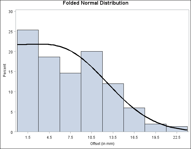
The following statements read the ANNOTATE= data set and display the histogram and fitted curve:

title 'Folded Normal Distribution';
ods graphics off;
proc univariate data=assembly noprint;
   histogram Offset / annotate = anno;
run;

Output 4.25.4 displays the histogram and fitted curve.

Output 4.25.4 Histogram with Annotated Folded Normal Curve

A sample program for this example, uniex15.sas, is available in the SAS Sample Library for Base SAS software.