The UNIVARIATE Procedure
- Overview
-
Getting Started

-
Syntax
-
Details
Missing Values Rounding Descriptive Statistics Calculating the Mode Calculating Percentiles Tests for Location Confidence Limits for Parameters of the Normal Distribution Robust Estimators Creating Line Printer Plots Creating High-Resolution Graphics Using the CLASS Statement to Create Comparative Plots Positioning Insets Formulas for Fitted Continuous Distributions Goodness-of-Fit Tests Kernel Density Estimates Construction of Quantile-Quantile and Probability Plots Interpretation of Quantile-Quantile and Probability Plots Distributions for Probability and Q-Q Plots Estimating Shape Parameters Using Q-Q Plots Estimating Location and Scale Parameters Using Q-Q Plots Estimating Percentiles Using Q-Q Plots Input Data Sets OUT= Output Data Set in the OUTPUT Statement OUTHISTOGRAM= Output Data Set OUTKERNEL= Output Data Set OUTTABLE= Output Data Set Tables for Summary Statistics ODS Table Names ODS Tables for Fitted Distributions ODS Graphics Computational Resources
-
Examples
Computing Descriptive Statistics for Multiple Variables Calculating Modes Identifying Extreme Observations and Extreme Values Creating a Frequency Table Creating Plots for Line Printer Output Analyzing a Data Set With a FREQ Variable Saving Summary Statistics in an OUT= Output Data Set Saving Percentiles in an Output Data Set Computing Confidence Limits for the Mean, Standard Deviation, and Variance Computing Confidence Limits for Quantiles and Percentiles Computing Robust Estimates Testing for Location Performing a Sign Test Using Paired Data Creating a Histogram Creating a One-Way Comparative Histogram Creating a Two-Way Comparative Histogram Adding Insets with Descriptive Statistics Binning a Histogram Adding a Normal Curve to a Histogram Adding Fitted Normal Curves to a Comparative Histogram Fitting a Beta Curve Fitting Lognormal, Weibull, and Gamma Curves Computing Kernel Density Estimates Fitting a Three-Parameter Lognormal Curve Annotating a Folded Normal Curve Creating Lognormal Probability Plots Creating a Histogram to Display Lognormal Fit Creating a Normal Quantile Plot Adding a Distribution Reference Line Interpreting a Normal Quantile Plot Estimating Three Parameters from Lognormal Quantile Plots Estimating Percentiles from Lognormal Quantile Plots Estimating Parameters from Lognormal Quantile Plots Comparing Weibull Quantile Plots Creating a Cumulative Distribution Plot Creating a P-P Plot
- References
| Construction of Quantile-Quantile and Probability Plots |
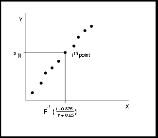
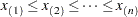
Figure 4.14 illustrates how a Q-Q plot is constructed for a specified theoretical distribution. First, the  nonmissing values of the variable are ordered from smallest to largest:
 |
Then the  th ordered value
  is plotted as a point whose
  -coordinate is and whose
  -coordinate is
  , where
  is the specified distribution with zero location parameter and unit scale parameter.
You can modify the adjustment constants  0.375 and 0.25 with the RANKADJ= and NADJ= options. This default combination is recommended by Blom (1958). For additional information, see Chambers et al. (1983). Because is a quantile of the empirical cumulative distribution function (ecdf), a Q-Q plot compares quantiles of the ecdf with quantiles of a theoretical distribution. Probability plots (see the section PROBPLOT Statement) are constructed the same way, except that the -axis is scaled nonlinearly in percentiles.