The UNIVARIATE Procedure
- Overview
-
Getting Started

-
Syntax
-
Details
Missing Values Rounding Descriptive Statistics Calculating the Mode Calculating Percentiles Tests for Location Confidence Limits for Parameters of the Normal Distribution Robust Estimators Creating Line Printer Plots Creating High-Resolution Graphics Using the CLASS Statement to Create Comparative Plots Positioning Insets Formulas for Fitted Continuous Distributions Goodness-of-Fit Tests Kernel Density Estimates Construction of Quantile-Quantile and Probability Plots Interpretation of Quantile-Quantile and Probability Plots Distributions for Probability and Q-Q Plots Estimating Shape Parameters Using Q-Q Plots Estimating Location and Scale Parameters Using Q-Q Plots Estimating Percentiles Using Q-Q Plots Input Data Sets OUT= Output Data Set in the OUTPUT Statement OUTHISTOGRAM= Output Data Set OUTKERNEL= Output Data Set OUTTABLE= Output Data Set Tables for Summary Statistics ODS Table Names ODS Tables for Fitted Distributions ODS Graphics Computational Resources
-
Examples
Computing Descriptive Statistics for Multiple Variables Calculating Modes Identifying Extreme Observations and Extreme Values Creating a Frequency Table Creating Plots for Line Printer Output Analyzing a Data Set With a FREQ Variable Saving Summary Statistics in an OUT= Output Data Set Saving Percentiles in an Output Data Set Computing Confidence Limits for the Mean, Standard Deviation, and Variance Computing Confidence Limits for Quantiles and Percentiles Computing Robust Estimates Testing for Location Performing a Sign Test Using Paired Data Creating a Histogram Creating a One-Way Comparative Histogram Creating a Two-Way Comparative Histogram Adding Insets with Descriptive Statistics Binning a Histogram Adding a Normal Curve to a Histogram Adding Fitted Normal Curves to a Comparative Histogram Fitting a Beta Curve Fitting Lognormal, Weibull, and Gamma Curves Computing Kernel Density Estimates Fitting a Three-Parameter Lognormal Curve Annotating a Folded Normal Curve Creating Lognormal Probability Plots Creating a Histogram to Display Lognormal Fit Creating a Normal Quantile Plot Adding a Distribution Reference Line Interpreting a Normal Quantile Plot Estimating Three Parameters from Lognormal Quantile Plots Estimating Percentiles from Lognormal Quantile Plots Estimating Parameters from Lognormal Quantile Plots Comparing Weibull Quantile Plots Creating a Cumulative Distribution Plot Creating a P-P Plot
- References
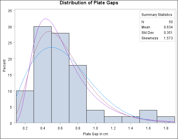
Example 4.22 Fitting Lognormal, Weibull, and Gamma Curves
To determine an appropriate model for a data distribution, you should consider curves from several distribution families. As shown in this example, you can use the HISTOGRAM statement to fit more than one distribution and display the density curves on a histogram.
The gap between two plates is measured (in cm) for each of 50 welded assemblies selected at random from the output of a welding process. The following statements save the measurements (Gap) in a data set named Plates:
data Plates;
   label Gap = 'Plate Gap in cm';
   input Gap @@;
   datalines;
0.746  0.357  0.376  0.327  0.485 1.741  0.241  0.777  0.768  0.409
0.252  0.512  0.534  1.656  0.742 0.378  0.714  1.121  0.597  0.231
0.541  0.805  0.682  0.418  0.506 0.501  0.247  0.922  0.880  0.344
0.519  1.302  0.275  0.601  0.388 0.450  0.845  0.319  0.486  0.529
1.547  0.690  0.676  0.314  0.736 0.643  0.483  0.352  0.636  1.080
;
The following statements fit three distributions (lognormal, Weibull, and gamma) and display their density curves on a single histogram:
title 'Distribution of Plate Gaps';
ods graphics off;
ods select ParameterEstimates GoodnessOfFit FitQuantiles MyHist;
proc univariate data=Plates;
   var Gap;
   histogram / midpoints=0.2 to 1.8 by 0.2
               lognormal
               weibull
               gamma
               vaxis   = axis1
               name    = 'MyHist';
   inset n mean(5.3) std='Std Dev'(5.3) skewness(5.3)
          / pos = ne  header = 'Summary Statistics';
   axis1 label=(a=90 r=0);
run;
The ODS SELECT statement restricts the output to the "ParameterEstimates," "GoodnessOfFit," and "FitQuantiles" tables; see the section ODS Table Names. The LOGNORMAL, WEIBULL, and GAMMA primary options request superimposed fitted curves on the histogram in Output 4.22.1. Note that a threshold parameter  is assumed for each curve. In applications where the threshold is not zero, you can specify
  with the THETA= secondary option.
The LOGNORMAL, WEIBULL, and GAMMA options also produce the summaries for the fitted distributions shown in Output 4.22.2 through Output 4.22.4.
Output 4.22.2 provides three EDF goodness-of-fit tests for the lognormal distribution: the Anderson-Darling, the Cramér-von Mises, and the Kolmogorov-Smirnov tests. At the  significance level, all tests support the conclusion that the two-parameter lognormal distribution with scale parameter
  and shape parameter
  provides a good model for the distribution of plate gaps.
| Distribution of Plate Gaps |
| Parameters for Lognormal Distribution | ||
|---|---|---|
| Parameter | Symbol | Estimate |
| Threshold | Theta | 0 |
| Scale | Zeta | -0.58375 |
| Shape | Sigma | 0.499546 |
| Mean | 0.631932 | |
| Std Dev | 0.336436 | |
| Goodness-of-Fit Tests for Lognormal Distribution | ||||
|---|---|---|---|---|
| Test | Statistic | p Value | ||
| Kolmogorov-Smirnov | D | 0.06441431 | Pr > D | >0.150 |
| Cramer-von Mises | W-Sq | 0.02823022 | Pr > W-Sq | >0.500 |
| Anderson-Darling | A-Sq | 0.24308402 | Pr > A-Sq | >0.500 |
| Quantiles for Lognormal Distribution | ||
|---|---|---|
| Percent | Quantile | |
| Observed | Estimated | |
| 1.0 | 0.23100 | 0.17449 |
| 5.0 | 0.24700 | 0.24526 |
| 10.0 | 0.29450 | 0.29407 |
| 25.0 | 0.37800 | 0.39825 |
| 50.0 | 0.53150 | 0.55780 |
| 75.0 | 0.74600 | 0.78129 |
| 90.0 | 1.10050 | 1.05807 |
| 95.0 | 1.54700 | 1.26862 |
| 99.0 | 1.74100 | 1.78313 |
| Distribution of Plate Gaps |
| Parameters for Weibull Distribution | ||
|---|---|---|
| Parameter | Symbol | Estimate |
| Threshold | Theta | 0 |
| Scale | Sigma | 0.719208 |
| Shape | C | 1.961159 |
| Mean | 0.637641 | |
| Std Dev | 0.339248 | |
| Goodness-of-Fit Tests for Weibull Distribution | ||||
|---|---|---|---|---|
| Test | Statistic | p Value | ||
| Cramer-von Mises | W-Sq | 0.15937281 | Pr > W-Sq | 0.016 |
| Anderson-Darling | A-Sq | 1.15693542 | Pr > A-Sq | <0.010 |
| Quantiles for Weibull Distribution | ||
|---|---|---|
| Percent | Quantile | |
| Observed | Estimated | |
| 1.0 | 0.23100 | 0.06889 |
| 5.0 | 0.24700 | 0.15817 |
| 10.0 | 0.29450 | 0.22831 |
| 25.0 | 0.37800 | 0.38102 |
| 50.0 | 0.53150 | 0.59661 |
| 75.0 | 0.74600 | 0.84955 |
| 90.0 | 1.10050 | 1.10040 |
| 95.0 | 1.54700 | 1.25842 |
| 99.0 | 1.74100 | 1.56691 |
Output 4.22.3 provides two EDF goodness-of-fit tests for the Weibull distribution: the Anderson-Darling and the Cramér-von Mises tests. The  -values for the EDF tests are all less than 0.10, indicating that the data do not support a Weibull model.
| Distribution of Plate Gaps |
| Parameters for Gamma Distribution | ||
|---|---|---|
| Parameter | Symbol | Estimate |
| Threshold | Theta | 0 |
| Scale | Sigma | 0.155198 |
| Shape | Alpha | 4.082646 |
| Mean | 0.63362 | |
| Std Dev | 0.313587 | |
| Goodness-of-Fit Tests for Gamma Distribution | ||||
|---|---|---|---|---|
| Test | Statistic | p Value | ||
| Kolmogorov-Smirnov | D | 0.09695325 | Pr > D | >0.250 |
| Cramer-von Mises | W-Sq | 0.07398467 | Pr > W-Sq | >0.250 |
| Anderson-Darling | A-Sq | 0.58106613 | Pr > A-Sq | 0.137 |
| Quantiles for Gamma Distribution | ||
|---|---|---|
| Percent | Quantile | |
| Observed | Estimated | |
| 1.0 | 0.23100 | 0.13326 |
| 5.0 | 0.24700 | 0.21951 |
| 10.0 | 0.29450 | 0.27938 |
| 25.0 | 0.37800 | 0.40404 |
| 50.0 | 0.53150 | 0.58271 |
| 75.0 | 0.74600 | 0.80804 |
| 90.0 | 1.10050 | 1.05392 |
| 95.0 | 1.54700 | 1.22160 |
| 99.0 | 1.74100 | 1.57939 |
significance level, all tests support the conclusion that the gamma distribution with scale parameter  and shape parameter
  provides a good model for the distribution of plate gaps.
 Based on this analysis, the fitted lognormal distribution and the fitted gamma distribution are both good models for the distribution of plate gaps.
A sample program for this example, uniex13.sas, is available in the SAS Sample Library for Base SAS software.