The UNIVARIATE Procedure
- Overview
-
Getting Started

-
Syntax
-
Details
Missing Values Rounding Descriptive Statistics Calculating the Mode Calculating Percentiles Tests for Location Confidence Limits for Parameters of the Normal Distribution Robust Estimators Creating Line Printer Plots Creating High-Resolution Graphics Using the CLASS Statement to Create Comparative Plots Positioning Insets Formulas for Fitted Continuous Distributions Goodness-of-Fit Tests Kernel Density Estimates Construction of Quantile-Quantile and Probability Plots Interpretation of Quantile-Quantile and Probability Plots Distributions for Probability and Q-Q Plots Estimating Shape Parameters Using Q-Q Plots Estimating Location and Scale Parameters Using Q-Q Plots Estimating Percentiles Using Q-Q Plots Input Data Sets OUT= Output Data Set in the OUTPUT Statement OUTHISTOGRAM= Output Data Set OUTKERNEL= Output Data Set OUTTABLE= Output Data Set Tables for Summary Statistics ODS Table Names ODS Tables for Fitted Distributions ODS Graphics Computational Resources
-
Examples
Computing Descriptive Statistics for Multiple Variables Calculating Modes Identifying Extreme Observations and Extreme Values Creating a Frequency Table Creating Plots for Line Printer Output Analyzing a Data Set With a FREQ Variable Saving Summary Statistics in an OUT= Output Data Set Saving Percentiles in an Output Data Set Computing Confidence Limits for the Mean, Standard Deviation, and Variance Computing Confidence Limits for Quantiles and Percentiles Computing Robust Estimates Testing for Location Performing a Sign Test Using Paired Data Creating a Histogram Creating a One-Way Comparative Histogram Creating a Two-Way Comparative Histogram Adding Insets with Descriptive Statistics Binning a Histogram Adding a Normal Curve to a Histogram Adding Fitted Normal Curves to a Comparative Histogram Fitting a Beta Curve Fitting Lognormal, Weibull, and Gamma Curves Computing Kernel Density Estimates Fitting a Three-Parameter Lognormal Curve Annotating a Folded Normal Curve Creating Lognormal Probability Plots Creating a Histogram to Display Lognormal Fit Creating a Normal Quantile Plot Adding a Distribution Reference Line Interpreting a Normal Quantile Plot Estimating Three Parameters from Lognormal Quantile Plots Estimating Percentiles from Lognormal Quantile Plots Estimating Parameters from Lognormal Quantile Plots Comparing Weibull Quantile Plots Creating a Cumulative Distribution Plot Creating a P-P Plot
- References
| Distributions for Probability and Q-Q Plots |
You can use the PROBPLOT and QQPLOT statements to request probability and Q-Q plots that are based on the theoretical distributions summarized in Table 4.116.
Parameters |
||||||
|---|---|---|---|---|---|---|
Distribution |
Density Function |
Range |
Location |
Scale |
Shape |
|
Beta |
|
|
|
|
|
|
Exponential |
|
|
|
|
||
Gamma |
|
|
|
|
|
|
Gumbel |
|
all |
|
|
||
Lognormal |
|
|
|
|
|
|
(3-parameter) |
||||||
Normal |
|
all |
|
|
||
Generalized |
|
|
|
|
|
|
Pareto |
|
|
||||
Power Function |
|
|
|
|
|
|
Rayleigh |
|
|
|
|
||
Weibull |
|
|
|
|
|
|
(3-parameter) |
||||||
Weibull |
|
|
|
|
|
|
(2-parameter) |
(known) |
|||||


You can request these distributions with the BETA, EXPONENTIAL, GAMMA, PARETO, GUMBEL, LOGNORMAL, NORMAL, POWER, RAYLEIGH, WEIBULL, and WEIBULL2 options, respectively. If you do not specify a distribution option, a normal probability plot or a normal Q-Q plot is created.
The following sections provide details for constructing Q-Q plots that are based on these distributions. Probability plots are constructed similarly except that the horizontal axis is scaled in percentile units.
Beta Distribution
To create the plot, the observations are ordered from smallest to largest, and the  th ordered observation is plotted against the quantile
  , where
  is the inverse normalized incomplete beta function,
  is the number of nonmissing observations, and
  and
and  are the shape parameters of the beta distribution. In a probability plot, the horizontal axis is scaled in percentile units.
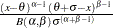
The pattern on the plot for ALPHA= and BETA= tends to be linear with intercept  and slope
  if the data are beta distributed with the specific density function
 |
where 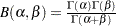 and
and
 lower threshold parameter
  scale parameter
 first shape parameter
 second shape parameter
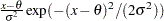
Exponential Distribution
To create the plot, the observations are ordered from smallest to largest, and the th ordered observation is plotted against the quantile 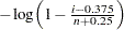 , where is the number of nonmissing observations. In a probability plot, the horizontal axis is scaled in percentile units.
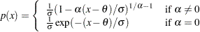
The pattern on the plot tends to be linear with intercept and slope if the data are exponentially distributed with the specific density function
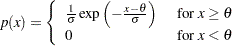 |
where is a threshold parameter, and is a positive scale parameter.
Gamma Distribution
To create the plot, the observations are ordered from smallest to largest, and the th ordered observation is plotted against the quantile  , where
  is the inverse normalized incomplete gamma function, is the number of nonmissing observations, and is the shape parameter of the gamma distribution. In a probability plot, the horizontal axis is scaled in percentile units.
The pattern on the plot for ALPHA= tends to be linear with intercept and slope if the data are gamma distributed with the specific density function
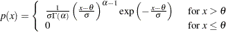 |
where
- threshold parameter
- scale parameter
- shape parameter
Gumbel Distribution
To create the plot, the observations are ordered from smallest to largest, and the th ordered observation is plotted against the quantile 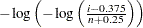 , where is the number of nonmissing observations. In a probability plot, the horizontal axis is scaled in percentile units.
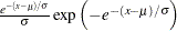
The pattern on the plot tends to be linear with intercept  and slope if the data are Gumbel distributed with the specific density function
 |
 location parameter
 - scale parameter
Lognormal Distribution
To create the plot, the observations are ordered from smallest to largest, and the th ordered observation is plotted against the quantile 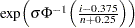 , where
  is the inverse cumulative standard normal distribution, is the number of nonmissing observations, and is the shape parameter of the lognormal distribution. In a probability plot, the horizontal axis is scaled in percentile units.
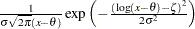
The pattern on the plot for SIGMA= tends to be linear with intercept and slope  if the data are lognormally distributed with the specific density function
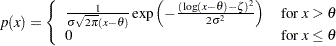 |
where
- threshold parameter
 scale parameter
 - shape parameter

See Example 4.26 and Example 4.33.
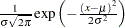
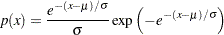
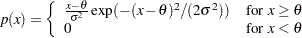
Normal Distribution
To create the plot, the observations are ordered from smallest to largest, and the th ordered observation is plotted against the quantile  , where is the inverse cumulative standard normal distribution and is the number of nonmissing observations. In a probability plot, the horizontal axis is scaled in percentile units.
The point pattern on the plot tends to be linear with intercept and slope if the data are normally distributed with the specific density function
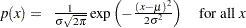 |
where is the mean and is the standard deviation ( ).
).
Generalized Pareto Distribution
To create the plot, the observations are ordered from smallest to largest, and the th ordered observation is plotted against the quantile 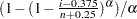 (
( ) or
) or 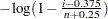 (
( ), where is the number of nonmissing observations and is the shape parameter of the generalized Pareto distribution. The horizontal axis is scaled in percentile units.
The point pattern on the plot for ALPHA= tends to be linear with intercept and slope if the data are generalized Pareto distributed with the specific density function
 |
where threshold parameter scale parameter shape parameter
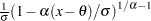
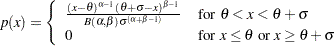
Power Function Distribution
To create the plot, the observations are ordered from smallest to largest, and the th ordered observation is plotted against the quantile  , where
  is the inverse normalized incomplete beta function, is the number of nonmissing observations, is one shape parameter of the beta distribution, and the second shape parameter,
  . The horizontal axis is scaled in percentile units.
The point pattern on the plot for ALPHA= tends to be linear with intercept and slope if the data are power function distributed with the specific density function
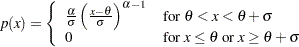 |
where
- threshold parameter
- shape parameter
- shape parameter

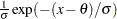
Rayleigh Distribution
To create the plot, the observations are ordered from smallest to largest, and the th ordered observation is plotted against the quantile 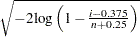 , where is the number of nonmissing observations. The horizontal axis is scaled in percentile units.
The point pattern on the plot tends to be linear with intercept and slope if the data are Rayleigh distributed with the specific density function
 |
where is a threshold parameter, and is a positive scale parameter.
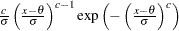
Three-Parameter Weibull Distribution
To create the plot, the observations are ordered from smallest to largest, and the th ordered observation is plotted against the quantile 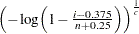 , where is the number of nonmissing observations, and
  is the Weibull distribution shape parameter. In a probability plot, the horizontal axis is scaled in percentile units.
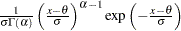
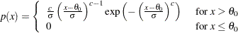
The pattern on the plot for C= tends to be linear with intercept and slope if the data are Weibull distributed with the specific density function
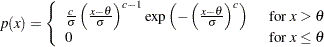 |
where
- threshold parameter
- scale parameter
 shape parameter
See Example 4.34.
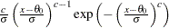
Two-Parameter Weibull Distribution
To create the plot, the observations are ordered from smallest to largest, and the log of the shifted th ordered observation  , denoted by
  , is plotted against the quantile
 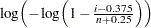 , where is the number of nonmissing observations. In a probability plot, the horizontal axis is scaled in percentile units.
Unlike the three-parameter Weibull quantile, the preceding expression is free of distribution parameters. Consequently, the C= shape parameter is not mandatory with the WEIBULL2 distribution option.
The pattern on the plot for THETA= tends to be linear with intercept
  and slope
  if the data are Weibull distributed with the specific density function
 |
where
 known lower threshold
 - scale parameter
- shape parameter

See Example 4.34.