The UNIVARIATE Procedure
- Overview
-
Getting Started

-
Syntax
-
Details
Missing Values Rounding Descriptive Statistics Calculating the Mode Calculating Percentiles Tests for Location Confidence Limits for Parameters of the Normal Distribution Robust Estimators Creating Line Printer Plots Creating High-Resolution Graphics Using the CLASS Statement to Create Comparative Plots Positioning Insets Formulas for Fitted Continuous Distributions Goodness-of-Fit Tests Kernel Density Estimates Construction of Quantile-Quantile and Probability Plots Interpretation of Quantile-Quantile and Probability Plots Distributions for Probability and Q-Q Plots Estimating Shape Parameters Using Q-Q Plots Estimating Location and Scale Parameters Using Q-Q Plots Estimating Percentiles Using Q-Q Plots Input Data Sets OUT= Output Data Set in the OUTPUT Statement OUTHISTOGRAM= Output Data Set OUTKERNEL= Output Data Set OUTTABLE= Output Data Set Tables for Summary Statistics ODS Table Names ODS Tables for Fitted Distributions ODS Graphics Computational Resources
-
Examples
Computing Descriptive Statistics for Multiple Variables Calculating Modes Identifying Extreme Observations and Extreme Values Creating a Frequency Table Creating Plots for Line Printer Output Analyzing a Data Set With a FREQ Variable Saving Summary Statistics in an OUT= Output Data Set Saving Percentiles in an Output Data Set Computing Confidence Limits for the Mean, Standard Deviation, and Variance Computing Confidence Limits for Quantiles and Percentiles Computing Robust Estimates Testing for Location Performing a Sign Test Using Paired Data Creating a Histogram Creating a One-Way Comparative Histogram Creating a Two-Way Comparative Histogram Adding Insets with Descriptive Statistics Binning a Histogram Adding a Normal Curve to a Histogram Adding Fitted Normal Curves to a Comparative Histogram Fitting a Beta Curve Fitting Lognormal, Weibull, and Gamma Curves Computing Kernel Density Estimates Fitting a Three-Parameter Lognormal Curve Annotating a Folded Normal Curve Creating Lognormal Probability Plots Creating a Histogram to Display Lognormal Fit Creating a Normal Quantile Plot Adding a Distribution Reference Line Interpreting a Normal Quantile Plot Estimating Three Parameters from Lognormal Quantile Plots Estimating Percentiles from Lognormal Quantile Plots Estimating Parameters from Lognormal Quantile Plots Comparing Weibull Quantile Plots Creating a Cumulative Distribution Plot Creating a P-P Plot
- References
Example 4.15 Creating a One-Way Comparative Histogram
This example illustrates how to create a comparative histogram. The effective channel length (in microns) is measured for 1225 field effect transistors. The channel lengths (Length) are stored in a data set named Channel, which is partially listed in Output 4.15.1:
| The Data Set Channel |
| Lot | Length |
|---|---|
| Lot 1 | 0.91 |
| . | . |
| Lot 1 | 1.17 |
| Lot 2 | 1.47 |
| . | . |
| Lot 2 | 1.39 |
| Lot 3 | 2.04 |
| . | . |
| Lot 3 | 1.91 |
The following statements request a histogram of Length ignoring the lot source:
title 'Histogram of Length Ignoring Lot Source';
ods graphics off;
proc univariate data=Channel noprint;
   histogram Length;
run;
The resulting histogram is shown in Output 4.15.2.
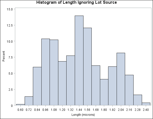
To investigate whether the peaks (modes) in Output 4.15.2 are related to the lot source, you can create a comparative histogram by using Lot as a classification variable. The following statements create the histogram shown in Output 4.15.3:
title 'Comparative Analysis of Lot Source';
ods graphics off;
proc univariate data=Channel noprint;
   class Lot;
   histogram Length / nrows = 3;
run;
The CLASS statement requests comparisons for each level (distinct value) of the classification variable Lot. The HISTOGRAM statement requests a comparative histogram for the variable Length. The NROWS= option specifies the number of rows per panel in the comparative histogram. By default, comparative histograms are displayed in two rows per panel.
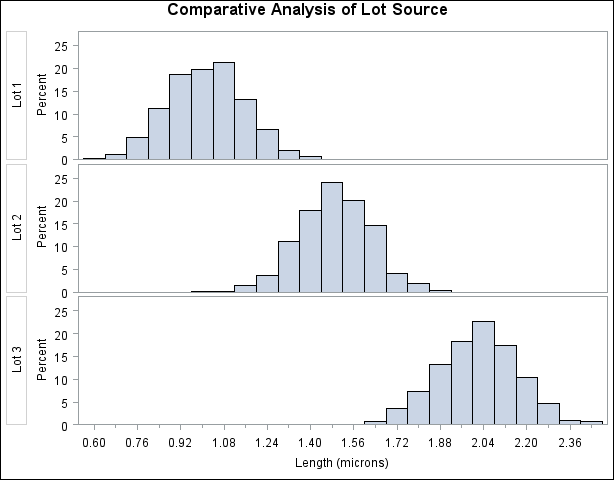
Output 4.15.3 reveals that the distributions of Length are similarly distributed except for shifts in mean.
A sample program for this example, uniex09.sas, is available in the SAS Sample Library for Base SAS software.