The UNIVARIATE Procedure
- Overview
-
Getting Started

-
Syntax
-
Details
Missing Values Rounding Descriptive Statistics Calculating the Mode Calculating Percentiles Tests for Location Confidence Limits for Parameters of the Normal Distribution Robust Estimators Creating Line Printer Plots Creating High-Resolution Graphics Using the CLASS Statement to Create Comparative Plots Positioning Insets Formulas for Fitted Continuous Distributions Goodness-of-Fit Tests Kernel Density Estimates Construction of Quantile-Quantile and Probability Plots Interpretation of Quantile-Quantile and Probability Plots Distributions for Probability and Q-Q Plots Estimating Shape Parameters Using Q-Q Plots Estimating Location and Scale Parameters Using Q-Q Plots Estimating Percentiles Using Q-Q Plots Input Data Sets OUT= Output Data Set in the OUTPUT Statement OUTHISTOGRAM= Output Data Set OUTKERNEL= Output Data Set OUTTABLE= Output Data Set Tables for Summary Statistics ODS Table Names ODS Tables for Fitted Distributions ODS Graphics Computational Resources
-
Examples
Computing Descriptive Statistics for Multiple Variables Calculating Modes Identifying Extreme Observations and Extreme Values Creating a Frequency Table Creating Plots for Line Printer Output Analyzing a Data Set With a FREQ Variable Saving Summary Statistics in an OUT= Output Data Set Saving Percentiles in an Output Data Set Computing Confidence Limits for the Mean, Standard Deviation, and Variance Computing Confidence Limits for Quantiles and Percentiles Computing Robust Estimates Testing for Location Performing a Sign Test Using Paired Data Creating a Histogram Creating a One-Way Comparative Histogram Creating a Two-Way Comparative Histogram Adding Insets with Descriptive Statistics Binning a Histogram Adding a Normal Curve to a Histogram Adding Fitted Normal Curves to a Comparative Histogram Fitting a Beta Curve Fitting Lognormal, Weibull, and Gamma Curves Computing Kernel Density Estimates Fitting a Three-Parameter Lognormal Curve Annotating a Folded Normal Curve Creating Lognormal Probability Plots Creating a Histogram to Display Lognormal Fit Creating a Normal Quantile Plot Adding a Distribution Reference Line Interpreting a Normal Quantile Plot Estimating Three Parameters from Lognormal Quantile Plots Estimating Percentiles from Lognormal Quantile Plots Estimating Parameters from Lognormal Quantile Plots Comparing Weibull Quantile Plots Creating a Cumulative Distribution Plot Creating a P-P Plot
- References
Example 4.19 Adding a Normal Curve to a Histogram
This example is a continuation of Example 4.14. The following statements fit a normal distribution to the thickness measurements in the Trans data set and superimpose the fitted density curve on the histogram:
title 'Analysis of Plating Thickness';
ods graphics off;
ods select ParameterEstimates GoodnessOfFit FitQuantiles Bins MyPlot;
proc univariate data=Trans;
   histogram Thick / normal(percents=20 40 60 80 midpercents)
                     name='MyPlot';
   inset n normal(ksdpval) / pos = ne format = 6.3;
run;
The ODS SELECT statement restricts the output to the "ParameterEstimates," "GoodnessOfFit," "FitQuantiles," and "Bins" tables; see the section ODS Table Names. The NORMAL option specifies that the normal curve be displayed on the histogram shown in Output 4.19.2. It also requests a summary of the fitted distribution, which is shown in Output 4.19.1. goodness-of-fit tests, parameter estimates, and quantiles of the fitted distribution. (If you specify the NORMALTEST option in the PROC UNIVARIATE statement, the Shapiro-Wilk test for normality is included in the tables of statistical output.)
Two secondary options are specified in parentheses after the NORMAL primary option. The PERCENTS= option specifies quantiles, which are to be displayed in the "FitQuantiles" table. The MIDPERCENTS option requests a table that lists the midpoints, the observed percentage of observations, and the estimated percentage of the population in each interval (estimated from the fitted normal distribution). See Table 4.17 and Table 4.24 for the secondary options that can be specified with after the NORMAL primary option.
| Analysis of Plating Thickness |
| Parameters for Normal Distribution | ||
|---|---|---|
| Parameter | Symbol | Estimate |
| Mean | Mu | 3.49533 |
| Std Dev | Sigma | 0.032117 |
| Goodness-of-Fit Tests for Normal Distribution | ||||
|---|---|---|---|---|
| Test | Statistic | p Value | ||
| Kolmogorov-Smirnov | D | 0.05563823 | Pr > D | >0.150 |
| Cramer-von Mises | W-Sq | 0.04307548 | Pr > W-Sq | >0.250 |
| Anderson-Darling | A-Sq | 0.27840748 | Pr > A-Sq | >0.250 |
| Histogram Bin Percents for Normal Distribution |
||
|---|---|---|
| Bin Midpoint |
Percent | |
| Observed | Estimated | |
| 3.43 | 3.000 | 3.296 |
| 3.45 | 9.000 | 9.319 |
| 3.47 | 23.000 | 18.091 |
| 3.49 | 19.000 | 24.124 |
| 3.51 | 24.000 | 22.099 |
| 3.53 | 15.000 | 13.907 |
| 3.55 | 3.000 | 6.011 |
| 3.57 | 4.000 | 1.784 |
| Quantiles for Normal Distribution | ||
|---|---|---|
| Percent | Quantile | |
| Observed | Estimated | |
| 20.0 | 3.46700 | 3.46830 |
| 40.0 | 3.48350 | 3.48719 |
| 60.0 | 3.50450 | 3.50347 |
| 80.0 | 3.52250 | 3.52236 |
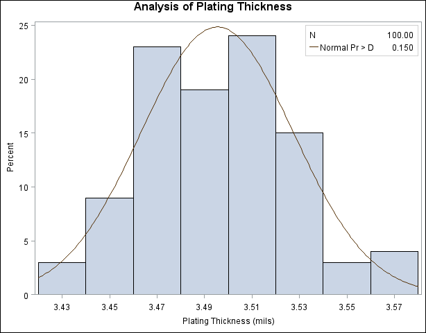
The histogram of the variable Thick with a superimposed normal curve is shown in Output 4.19.2.
The estimated parameters for the normal curve ( and
and  ) are shown in Output 4.19.1. By default, the parameters are estimated unless you specify values with the MU= and SIGMA= secondary options after the NORMAL primary option. The results of three goodness-of-fit tests based on the empirical distribution function (EDF) are displayed in Output 4.19.1. Because the
  -values are all greater than 0.15, the hypothesis of normality is not rejected.
A sample program for this example, uniex08.sas, is available in the SAS Sample Library for Base SAS software.