The NLMIXED Procedure
-
Overview

-
Getting Started
-
Syntax
-
DetailsModeling Assumptions and NotationIntegral ApproximationsBuilt-in Log-Likelihood FunctionsHierarchical Model SpecificationOptimization AlgorithmsFinite-Difference Approximations of DerivativesHessian ScalingActive Set MethodsLine-Search MethodsRestricting the Step LengthComputational ProblemsCovariance MatrixPredictionComputational ResourcesDisplayed OutputODS Table Names
-
Examples
- References
Example 82.7 Overdispersion Hierarchical Nonlinear Mixed Model
This example describes the overdispersion hierarchical nonlinear mixed model that is given in Ghebretinsae et al. (2013). In this experiment, 24 rats are divided into four groups and receive a daily oral dose of 1,2-dimethylhydrazine dihydrochloride
in three dose levels (low, medium, and high) and a vehicle control. In addition, an extra group of three animals receive a
positive control. All 27 animals are euthanized 3 hours after the last dose is administered. For each animal, a cell suspension
is prepared, and from each cell suspension, three replicate samples are prepared for scoring. Using a semi-automated scoring
system, 50 randomly selected cells from each sample are scored per animal for DNA damage. The comet assay methodology is used
to detect this DNA damage. In this methodology, the DNA damage is measured by the distance of DNA migration from the perimeter
of the comet head to the last visible point in the tail. This distance is defined as the tail length and is observed for the
150 cells from each animal. The data are available in the Sashelp library. In order to use the dose levels as regressors in PROC NLMIXED, you need to create indicator variables for each dose
level. The following DATA step creates indicator variables for the dose levels:
data comet;
   set sashelp.comet;
   L = 0; M = 0; H = 0; PC = 0;
   if (dose = 1.25) then L  = 1;
   if (dose = 2.50) then M  = 1;
   if (dose = 5.00) then H  = 1;
   if (dose = 200)  then PC = 1;
run;
Ghebretinsae et al. (2013) suggest a Weibull distribution to model the outcomes (tail lengths). Note that the data exhibit the nested nature because
of the three replicate samples from each cell. Also, the 50 cells from each rat are correlated. To account for the dependency
of these 150 correlated cells from each rat, two levels of normally distributed nested random effects are used. Let  be the tail length that is observed in the kth cell from the jth sample of the ith rat. Then the suggested two-level nested model can be described as follows:
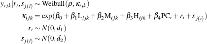
This model is referred to as the nested Weibull model in the rest of the example. The parameters of the Weibull distribution,
 and
and  , are known as the shape and scale parameters, respectively. Based on this model specification, the conditional expectation
of the response variable, given the random effects, is a nonlinear function of fixed and random effects. The nonlinear relationship
can be written as
, are known as the shape and scale parameters, respectively. Based on this model specification, the conditional expectation
of the response variable, given the random effects, is a nonlinear function of fixed and random effects. The nonlinear relationship
can be written as
These expected values can be obtained using the PREDICT statement in PROC NLMIXED, and they are useful for validating the model fitting. The specified nested Weibull model can be fitted using the following PROC NLMIXED statements:
proc nlmixed data = comet;
   parms b0 = -25  b1 = -10 b2 = -10 b3 = -10 b4 = -10 rho = 10;
   bounds sd1 >=0, sd2 >=0;
   mu = b0+ b1*L+ b2*M+ b3*H+ b4*PC + rateff + sampeff;
   term = (length**rho)*exp(mu);
   llike = log(rho) + (rho-1)*log(length) + mu - term;
   model length ~ general(llike);
   random ratEff ~ normal(0,sd1) subject = rat;
   random sampEff ~ normal(0,sd2) subject = sample(rat);
   predict gamma(1+(1/rho))/(exp(mu)**(1/rho)) out = p1;
run;
Note that the two-parameter Weibull density function is given by
![\[ f(y;\rho ,\kappa ) = \kappa \rho y^{\rho -1}e^{-\kappa y^{\rho }} \]](images/statug_nlmixed0380.png)
This implies that the log likelihood is
![\[ l(\rho ,\kappa ;y) = \log (\kappa ) + \log (\rho ) + (\rho -1)\log (y) -\kappa y^{\rho } \]](images/statug_nlmixed0381.png)
A general log-likelihood specification is used in the MODEL statement to specify the preceding log of the Weibull density.
The linear combination of the parameters, b to
to b , and the two random effects,
 RatEff and SampEff, is defined using the linear predictor MU in the first SAS programming statement. Then, the next two SAS programming statements
together define the log of the Weibull density function. The first RANDOM statement defines the first level of the random
effect,  , by using
 RatEff. Then, the second RANDOM statement defines the second level of the random effect,  , nested within the first level by using
 SampEff. Both random-effects distributions are specified as normal with mean 0 and variance sd1 and sd2 for the first and second levels, respectively. The selected output from this model is shown in Output 82.7.1, Output 82.7.2, and Output 82.7.3.
Output 82.7.1: Model Specification for Nested Weibull Model
| Specifications | |
|---|---|
| Data Set | WORK.COMET |
| Dependent Variable | Length |
| Distribution for Dependent Variable | General |
| Random Effects | rateff, sampeff |
| Distribution for Random Effects | Normal, Normal |
| Subject Variables | Rat, Sample |
| Optimization Technique | Dual Quasi-Newton |
| Integration Method | Adaptive Gaussian Quadrature |
The "Specifications" table shows that RatEff is the first-level random effect, specified by the subject variable Rat, and it follows a normal distribution (Output 82.7.1). Similarly, SampEff is the second-level random effect, nested in RatEff and specified by the subject variable Sample, and it follows a normal distribution.
Output 82.7.2: Dimensions Table for Nested Weibull Model
The "Dimensions" table indicates that 4,050 observations are used in the analysis (Output 82.7.2). It also indicates that there are 27 rats and that 81 samples are nested within the rats. As explained earlier, three samples are selected randomly from each rat, so a total of 81 (27 times 3) samples are used in the analysis.
Output 82.7.3: Parameter Estimates for Nested Weibull Model
| Parameter Estimates | ||||||||
|---|---|---|---|---|---|---|---|---|
| Parameter | Estimate | Standard Error |
DF | t Value | Pr > |t| | 95% Confidence Limits | Gradient | |
| b0 | -15.6346 | 0.2627 | 79 | -59.52 | <.0001 | -16.1575 | -15.1117 | -0.21455 |
| b1 | -4.4912 | 0.2345 | 79 | -19.15 | <.0001 | -4.9581 | -4.0244 | -0.12563 |
| b2 | -4.5865 | 0.2186 | 79 | -20.98 | <.0001 | -5.0216 | -4.1514 | 0.20926 |
| b3 | -4.8188 | 0.2188 | 79 | -22.02 | <.0001 | -5.2543 | -4.3833 | 0.088666 |
| b4 | -3.4834 | 0.2664 | 79 | -13.08 | <.0001 | -4.0136 | -2.9532 | -0.18096 |
| rho | 4.9558 | 0.05881 | 79 | 84.27 | <.0001 | 4.8388 | 5.0729 | -1.18121 |
| sd1 | 0.02454 | 0.04601 | 79 | 0.53 | 0.5953 | -0.06704 | 0.1161 | -0.75888 |
| sd2 | 0.3888 | 0.07106 | 79 | 5.47 | <.0001 | 0.2473 | 0.5302 | -0.79003 |
The "Parameter Estimates" table list the maximum likelihood estimates of the parameters along with their standard errors (Output 82.7.3). The estimates are fairly close to the estimates that are given in Ghebretinsae et al. (2013), who use a gamma distribution for the Sample random effects instead of the normal distribution as in the preceding model. Note that the parameters  ,
,  , and
, and  represent the effects of low, medium, and high doses, respectively, when compared to the vehicle control. Similarly,
  is the parameter that corresponds to the effect of positive control when compared to vehicle control. The p-value indicates that the point estimates of all these parameters, to , are significant; this implies that the toxicity of 1,2-dimethylhydrazine dihydrochloride is significant at different dose
levels.
is the parameter that corresponds to the effect of positive control when compared to vehicle control. The p-value indicates that the point estimates of all these parameters, to , are significant; this implies that the toxicity of 1,2-dimethylhydrazine dihydrochloride is significant at different dose
levels.
In the nested Weibull model, the scale parameter, , is random because it is a function of random effects. This implies that the model assumes that each observation is drawn
from a different Weibull distribution. Molenberghs et al. (2010) indicate that this way of modeling leads to an overdispersed Weibull model. Ghebretinsae et al. (2013) use the random-effects mechanism to account for this overdispersion. The overdispersed Weibull model can be written as follows:
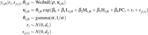
This model is referred to as the nested Weibull overdispersion model in the rest of this example. Again, in this model, the
shape parameter, , is the function of the normally distributed random effects, and , along with other random effects,  . Further, the model assumes that follow a gamma distribution. Note that the random effects, and , account for the cluster effect of the observations from the same sample that is nested within a rat, whereas account for the overdispersion in the data. Molenberghs et al. (2010) integrate out the overdispersion random effects, , from the joint distribution
  and provide the conditional density of
  . The conditional density follows:
Again, in this case, the conditional expectation of the response variable, given the random effects, is a nonlinear function of the fixed and random effects. Molenberghs et al. (2010) provide this nonlinear relationship as follows:
As indicated previously, these values are useful for validating the fit of the model, and they can be obtained using a PREDICT statement in PROC NLMIXED. Using the preceding conditional distribution of response, given the random effects and the random-effects distribution, PROC NLMIXED fits the two-level nested Weibull overdispersion model by using the following statements:
ods select ParameterEstimates;
proc nlmixed data = comet;
   parms b0 = -25  b1 = -10 b2 = -10 b3 = -10 b4 = -10 alpha = 1 rho = 10;
   bounds sd1 >=0, sd2 >=0;
   mu = b0+ b1*L+ b2*M+ b3*H+ b4*PC + rateff + sampeff;
   num = rho*((length)**(rho-1))*exp(mu);
   den = (1+(((length)**rho)*exp(mu))/alpha)**(alpha+1);
   llike = log(num/den);
   model length ~ general(llike);
   random rateff ~ normal(0,sd1) subject = rat;
   random sampeff ~ normal(0,sd2) subject = sample(rat);
   predict (gamma(alpha-(1/rho))*gamma(1+(1/rho)))
           /(gamma(alpha)*((exp(mu)/alpha)**(1/rho))) out = p2;
run;
The parameter estimates that are obtained from the nested Weibull overdispersion model are given in Output 82.7.1. The "Parameter Estimates" table indicates that the point estimates are still significant, as they are in the previous model in which the overdispersion is not taken into consideration. So the same conclusion about the dose levels holds: the toxicity of 1,2-dimethylhydrazine dihydrochloride is significant at different dose levels.
Output 82.7.4: Parameter Estimates for Nested Weibull Overdispersion Model
| Parameter Estimates | ||||||||
|---|---|---|---|---|---|---|---|---|
| Parameter | Estimate | Standard Error |
DF | t Value | Pr > |t| | 95% Confidence Limits | Gradient | |
| b0 | -31.0041 | 0.8155 | 79 | -38.02 | <.0001 | -32.6272 | -29.3810 | -0.27124 |
| b1 | -11.9102 | 0.5159 | 79 | -23.09 | <.0001 | -12.9371 | -10.8833 | -0.00736 |
| b2 | -12.1194 | 0.5173 | 79 | -23.43 | <.0001 | -13.1492 | -11.0897 | 0.095998 |
| b3 | -12.5516 | 0.5217 | 79 | -24.06 | <.0001 | -13.5900 | -11.5132 | 0.29527 |
| b4 | -9.6307 | 0.5554 | 79 | -17.34 | <.0001 | -10.7362 | -8.5251 | -0.12589 |
| alpha | 0.8925 | 0.05047 | 79 | 17.68 | <.0001 | 0.7920 | 0.9930 | 1.84146 |
| rho | 10.7188 | 0.2792 | 79 | 38.39 | <.0001 | 10.1632 | 11.2745 | -0.04855 |
| sd1 | 0.1908 | 0.1549 | 79 | 1.23 | 0.2217 | -0.1175 | 0.4990 | 0.49983 |
| sd2 | 0.7926 | 0.1666 | 79 | 4.76 | <.0001 | 0.4609 | 1.1242 | -0.04111 |
Recall that, from both models, the conditional expected values of the response variable, given the random effects, are obtained
using the PREDICT statement. These predicted values are stored in the data sets p1 and p2 for the nested Weibull and nested Weibull overdispersion models, respectively. Because, in this example, the regressor variables
are only indicators, the prediction values for all the observations from the same sample that is nested within a rat are equal.
Further, compute the average predicted value for each sample that is nested within a rat for both models. These values predict
the average tail length of each sample that is nested within a rat based on the fitted model. In addition, compute the observed
sample averages of the responses from each cluster, which can be viewed as the crude estimate of the average population tail
length for each cluster. The following statements combine all these average tail lengths, both observed and predicted, from
the two fitted models into a single data set:
proc means data = p1 mean noprint;
   class sample;
   var pred;
   output out = p11 (keep = sample weibull_mean)mean = weibull_mean;
run;

proc means data = p2 mean noprint;
   class sample;
   var pred;
   output out = p21 (keep = sample weibull_gamma_mean)mean = weibull_gamma_mean;
run;

proc means data = comet mean noprint;
   class sample;
   var length;
   id dose rat;
   output out = p31(keep = dose rat sample observed_mean) mean = observed_mean;
run;

data average;
   merge p11 p21 p31;
   by sample;
   if sample = . then delete;
   label observed_mean = "Observed Average";
   label weibull_gamma_mean = "Weibull Gamma Average";
   label weibull_mean = "Weibull Average";
   label sample = "Sample Index";
   if dose = 0 then dosage = "0 Vehicle Control ";
   if dose = 1.25 then dosage = "1 Low";
   if dose = 2.50 then dosage = "2 Medium";
   if dose = 5.00 then dosage = "3 High";
   if dose = 200  then dosage = "4 Positive Control";
run;
In order to validate the fit of the models, the observed average tail length values are plotted along with predicted average tail lengths from each model that is fitted using PROC NLMIXED. Moreover, the plots are created for each dosage level by using a PANELBY statement in PROC SGPANEL. The code follows:
proc sgpanel data = average;
   panelby dosage/onepanel layout = columnlattice novarname uniscale = row;
   rowaxis values=(10 to 80 by 5) label="Average Tail Length";
   series x = sample y = observed_mean;
   series x = sample y = weibull_mean;
   series x = sample y = weibull_gamma_mean;
run;
The resulting plots are given in Output 82.7.5.
Output 82.7.5: Comparison of Nested Weibull Model and Nested Weibull Overdispersion Model
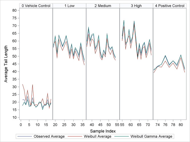
You can see from the plots that the observed averages of the tail lengths from each sample that is nested within a rat are closer to the predicted averages of the nested Weibull overdispersion model than to the predicted averages of the nested Weibull model.