The GAMPL Procedure
-
Overview

- Getting Started
-
Syntax
-
DetailsMissing ValuesThin-Plate Regression SplinesGeneralized Additive ModelsModel Evaluation CriteriaFitting AlgorithmsDegrees of FreedomModel InferenceDispersion ParameterTests for Smoothing ComponentsComputational Method: MultithreadingChoosing an Optimization TechniqueDisplayed OutputODS Table NamesODS Graphics
-
Examples
- References
Example 42.2 Nonparametric Logistic Regression
This example shows how you can use PROC GAMPL to build a nonparametric logistic regression model for a data set that contains a binary response and then use that model to classify observations.
The example uses the Pima Indian Diabetes data set, which can be obtained from the UCI Machine Learning Repository (Asuncion
and Newman 2007). It is extracted from a larger database that was originally owned by the National Institute of Diabetes and Digestive and
Kidney Diseases. Data are for female patients who are at least 21 years old, are of Pima Indian heritage, and live near Phoenix,
Arizona. The objective of this study is to investigate the relationship between a diabetes diagnosis and variables that represent
physiological measurements and medical attributes. Some missing or invalid observations are removed from the analysis. The
reduced data set contains 532 records. The following DATA step creates the data set Pima:
title 'Pima Indian Diabetes Study';
data Pima;
   input NPreg Glucose Pressure Triceps BMI Pedigree Age Diabetes Test@@;
   datalines;
 6  148  72  35  33.6  0.627  50  1  1    1   85  66  29  26.6  0.351  31  0  1
 1   89  66  23  28.1  0.167  21  0  0    3   78  50  32    31  0.248  26  1  0
 2  197  70  45  30.5  0.158  53  1  0    5  166  72  19  25.8  0.587  51  1  1
 0  118  84  47  45.8  0.551  31  1  1    1  103  30  38  43.3  0.183  33  0  1
 3  126  88  41  39.3  0.704  27  0  0    9  119  80  35    29  0.263  29  1  0

   ... more lines ...

 1  128  48  45  40.5  0.613  24  1  0    2  112  68  22  34.1  0.315  26  0  0
 1  140  74  26  24.1  0.828  23  0  1    2  141  58  34  25.4  0.699  24  0  1
 7  129  68  49  38.5  0.439  43  1  1    0  106  70  37  39.4  0.605  22  0  0
 1  118  58  36  33.3  0.261  23  0  1    8  155  62  26    34  0.543  46  1  0
;
The data set contains nine variables, including the binary response variable Diabetes. Table 42.15 describes the variables.
Table 42.15: Variables in the Pima Data Set
|
Variable |
Description |
|---|---|
|
|
Number of pregnancies |
|
|
Two-hour plasma glucose concentration in an oral glucose tolerance test |
|
|
Diastolic blood pressure (mm Hg) |
|
|
Triceps skin fold thickness (mm) |
|
|
Body mass index (weight in kg/(height in m) |
|
|
Diabetes pedigree function |
|
|
Age (years) |
|
|
0 if test negative for diabetes, 1 if test positive |
|
|
0 for training role, 1 for test |

The Test variable splits the data set into training and test subsets. The training observations (whose Test value is 0) hold approximately 59.4% of the data. To build a model that is based on the training data and evaluate its performance
by predicting the test data, you use the following statements to create a new variable, Result, whose value is the same as that of the Diabetes variable for a training observation and is missing for a test observation:
data Pima;
   set Pima;
   Result = Diabetes;
   if Test=1 then Result=.;
run;
As a starting point of your analysis, you can build a parametric logistic regression model on the training data and predict the test data. The following statements use PROC HPLOGISTIC to perform the analysis:
proc hplogistic data=Pima;
   model Diabetes(event='1') = NPreg Glucose Pressure Triceps
                               BMI Pedigree Age;
   partition role=Test(test='1' train='0');
run;
Output 42.2.1 shows the summary statistics from the parametric logistic regression model.
Output 42.2.1: Fit Statistics
Output 42.2.2 shows fit statistics for both training and test subsets of the data, including the misclassification error for the test data.
Output 42.2.2: Partition Fit Statistics
| Partition Fit Statistics | ||
|---|---|---|
| Statistic | Training | Testing |
| Area under the ROCC | 0.8607 | 0.8547 |
| Average Square Error | 0.1452 | 0.1401 |
| Hosmer-Lemeshow Test | 0.9726 | 0.1487 |
| Misclassification Error | 0.2061 | 0.2178 |
| R-Square | 0.3438 | 0.2557 |
| Max-rescaled R-Square | 0.4695 | 0.3706 |
| McFadden's R-Square | 0.3197 | 0.2522 |
| Mean Difference | 0.3780 | 0.3605 |
| Somers' D | 0.7213 | 0.7093 |
| True Negative Fraction | 0.8702 | 0.8435 |
| True Positive Fraction | 0.6639 | 0.6182 |
The parametric logistic regression model is restricted in the sense that all variables affect the response in strictly linear fashion. If you are uncertain that a variable is an important factor and its contribution is linear in predicting the response, you might want to choose a nonparametric logistic regression model to fit the data. You can use PROC GAMPL to form a nonparametric model by including the spline transformation of each explanatory variable, as shown in the following statements:
proc gampl data=Pima seed=12345;
   model Result(event='1') = spline(NPreg)    spline(Glucose)
                             spline(Pressure) spline(Triceps)
                             spline(BMI)      spline(Pedigree)
                             spline(Age) / dist=binary;
run;
Because the response variable Result is binary, the DIST=BINARY option in the MODEL statement specifies a binary distribution for the response variable. By default,
PROC GAMPL models the probability of the first ordered response category, which is a negative diabetes testing result in this
case. The EVENT=
option specifically requests that PROC GAMPL model the probability of positive diabetes testing results. The “Response Profile”
table in Output 42.2.3 shows the frequencies of the response in both categories.
Output 42.2.3: Response Profile
Output 42.2.4 lists the summary statistics from the nonparametric logistic regression model, which include spline transformations of all variables.
Output 42.2.4: Fit Statistics
The “Tests for Smoothing Components” table in Output 42.2.5 shows approximate tests results. Although some spline terms are significant, others are not. The null testing hypothesis
is whether the total contribution from a variable is 0. So you can form a reduced model by removing those nonsignificant spline
terms from the model. In this case, spline transformations for NPreg, Pressure, BMI, and Triceps are dropped from the model because their p-values are larger than the 0.1 nominal level.
Output 42.2.5: Tests for Smoothing Components
| Tests for Smoothing Components | ||||
|---|---|---|---|---|
| Component | Effective DF |
Effective DF for Test |
Chi-Square | Pr > ChiSq |
| Spline(NPreg) | 1.00001 | 1 | 0.0758 | 0.7831 |
| Spline(Glucose) | 1.00000 | 1 | 38.4662 | <.0001 |
| Spline(Pressure) | 7.80438 | 8 | 10.2605 | 0.2472 |
| Spline(Triceps) | 1.00000 | 1 | 0.6343 | 0.4258 |
| Spline(BMI) | 8.00000 | 8 | 11.8047 | 0.1601 |
| Spline(Pedigree) | 1.00002 | 1 | 8.5323 | 0.0035 |
| Spline(Age) | 5.05456 | 7 | 15.7671 | 0.0273 |
The following statements use PROC GAMPL to fit a reduced nonparametric logistic regression model. The OUTPUT statement requests
predicted probabilities for both training and test data sets. The ID statement requests that the Diabetes and Test variables also be included in the output data set so that you can use them to identify test observations and compute misclassification
errors.
ods graphics on;
proc gampl data=Pima plots seed=12345;
   model Result(event='1') = spline(Glucose)
                             spline(Pedigree) spline(Age) / dist=binary;
   output out=PimaOut;
   id Diabetes Test;
run;
Output 42.2.6 shows the summary statistics from the reduced nonparametric logistic regression model. The values of the information criteria are better than of the parametric logistic regression model.
Output 42.2.6: Fit Statistics
| Pima Indian Diabetes Study |
| Fit Statistics | |
|---|---|
| Penalized Log Likelihood | -149.85765 |
| Roughness Penalty | 2.85613 |
| Effective Degrees of Freedom | 8.05242 |
| Effective Degrees of Freedom for Error | 320.61181 |
| AIC (smaller is better) | 312.96402 |
| AICC (smaller is better) | 313.41826 |
| BIC (smaller is better) | 343.55593 |
| UBRE (smaller is better) | -0.00230 |
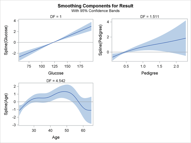
In the “Estimates for Smoothing Components” table in Output 42.2.7, PROC GAMPL reports that the effective degrees of freedom value for spline transformations of Glucose is quite close to 1. This suggests strictly linear form for Glucose. For Pedigree, the degrees of freedom value demonstrates a moderate amount of nonlinearity. For Age, the degrees of freedom value is much larger than 1. The measure suggests a nonlinear pattern in the dependency of the response
on Age.
Output 42.2.7: Estimates for Smoothing Components
The “Tests for Smoothing Components” table in Output 42.2.8 shows that all spline transformations are significant in predicting diabetes testing results.
Output 42.2.8: Tests for Smoothing Components
The smoothing component panel (which is produced by the PLOTS option and is shown in Output 42.2.9) visualizes the spline transformations for the four variables in addition to 95% Bayesian curvewise confidence bands. For
Glucose, the spline transformation is almost a straight line. For Pedigree, the spline transformation shows a slightly nonlinear trend. For Age, the dependency is obviously nonlinear.
Output 42.2.9: Smoothing Components Panel
The following statements compute the misclassification error on the test data set from the reduced nonparametric logistic regression model that PROC GAMPL produces:
data test;
   set PimaOut(where=(Test=1));
   if ((Pred>0.5 & Diabetes=1) | (Pred<0.5 & Diabetes=0))
   then Error=0;
   else Error=1;
run;

proc freq data=test;
   tables Diabetes*Error/nocol norow;
run;
Output 42.2.10 shows the misclassification errors for observations in the test set and observations of each response category. The error is smaller than the error from the parametric logistic regression model.
Output 42.2.10: Crosstabulation Table for Test Set Prediction