The GAMPL Procedure
-
Overview

- Getting Started
-
Syntax
-
DetailsMissing ValuesThin-Plate Regression SplinesGeneralized Additive ModelsModel Evaluation CriteriaFitting AlgorithmsDegrees of FreedomModel InferenceDispersion ParameterTests for Smoothing ComponentsComputational Method: MultithreadingChoosing an Optimization TechniqueDisplayed OutputODS Table NamesODS Graphics
-
Examples
- References
Thin-Plate Regression Splines
The GAMPL procedure uses thin-plate regression splines (Wood 2003) to construct spline basis expansions. The thin-plate regression splines are based on thin-plate smoothing splines (Duchon 1976, 1977). Compared to thin-plate smoothing splines, thin-plate regression splines produce fewer basis expansions and thus make direct fitting of generalized additive models possible.
Thin-Plate Smoothing Splines
Consider the problem of estimating a smoothing function f of  with d covariates from n observations. The model assumes
![\[ y_ i = f(\mb{x}_ i)+\epsilon _ i, i=1, \dots , n \]](images/statug_hpgam0051.png)
Then the thin-plate smoothing splines estimate the smoothing function f by minimizing the penalized least squares function:
![\[ \sum _{i=1}^ n (y_ i-f(\mb{x}_ i))^2 + \lambda J_{m,d}(f) \]](images/statug_hpgam0052.png)
The penalty term  includes the function that measures roughness on the f estimate:
![\[ J_{m,d}(f)= \int \cdots \int \sum _{\alpha _1+\cdots +\alpha _ d=m} \frac{m!}{\alpha _1!\cdots \alpha _ d !} \left( \begin{array}{c} \frac{\partial ^ m f}{\partial {x_1}^{\alpha _1}\cdots \partial {x_ d}^{\alpha _ d}} \end{array}\right)^2 \, \mr{d}x_1\cdots \mr{d}x_ d \]](images/statug_hpgam0054.png)
The parameter m (which corresponds to the M=
option for a spline effect) specifies how the penalty is applied to the function roughness. Function derivatives whose order
is less than m are not penalized. The relation  must be satisfied.
The penalty term also includes the smoothing parameter  , which controls the trade-off between the model’s fidelity to the data and the function smoothness of f. When
  , the function estimate corresponds to an interpolation. When
  , the function estimate becomes the least squares fit. By using the defined penalized least squares criterion and a fixed
 value, you can explicitly express the estimate of the smooth function f in the following form:
![\[ f_{\lambda }(\mb{x}) = \sum _{j=1}^ M\theta _ j\phi _ j(\mb{x})+\sum _ i^ n\delta _ i\eta _{m,d}(\| \mb{x}-\mb{x}_ i\| ) \]](images/statug_hpgam0060.png)
In the expression of  ,
,  and
and  are coefficients to be estimated. The functions
  correspond to unpenalized polynomials of with degrees up to
  . The total number of these polynomials is
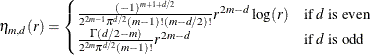
  . The function
  models the extra nonlinearity besides the polynomials and is a function of the Euclidean distance r between any value and an observed
  value:
Define the penalty matrix  such that each entry
 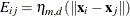 , let
, let  be the vector of the response, let
  be the matrix where each row is formed by , and let
  and
and  be vectors of coefficients and . Then you can obtain the function estimate
  from the following minimization problem:
![\[ \min \| \mb{y}-\bT \btheta -\bE \bdelta \| ^2+\lambda \bdelta ’\bE \bdelta \quad \text {subject to} \quad \bT ’\bdelta =\mb{0} \]](images/statug_hpgam0077.png)
For more information about thin-plate smoothing splines, see Chapter 116: The TPSPLINE Procedure.
Low-Rank Approximation
Given the representation of the thin-plate smoothing spline, the estimate of f involves as many parameters as the number of unique data points. Solving  with an optimum becomes difficult for large problems.
Because the matrix is symmetric and nonnegative definite, the eigendecomposition can be taken as  , where
  is the diagonal matrix of eigenvalues
  of , and
  is the matrix of eigenvectors that corresponds to
  . The truncated eigendecomposition forms
  , which is an approximation to such that
![\[ \tilde{\bE }_ k = \bU _ k \bD _ k \bU _ k’ \]](images/statug_hpgam0085.png)
where  is a diagonal matrix that contains the k most extreme eigenvalues in descending order of absolute values:
  .
.  is the matrix that is formed by columns of eigenvectors that correspond to the eigenvalues in .
The approximation not only reduces the dimension from  of to
of to  but also is optimal in two senses. First, minimizes the spectral norm
  between and all rank k matrices
  . Second, also minimizes the worst possible change that is introduced by the eigenspace truncation as defined by
![\[ \max _{\bdelta \ne \mb{0}} \frac{\bdelta '(\bE -\bG _ k)\bdelta }{\| \bdelta \| ^2} \]](images/statug_hpgam0093.png)
where  is formed by any k eigenvalues and corresponding eigenvectors. For more information, see Wood (2003).
Now given  and
and  , and letting
  , the minimization problem becomes
![\[ \min \| \mb{y}-\bT \btheta -\bU _ k\bD _ k\bdelta _ k\| ^2+\lambda \bdelta _ k’\bD _ k\bdelta _ k \quad \text {subject to} \quad \bT ’\bU _ k\bdelta _ k=\mb{0} \]](images/statug_hpgam0098.png)
You can turn the constrained optimization problem into an unconstrained one by using any orthogonal column basis  . One way to form is via the QR decomposition of
  :
:
![\[ \bU _ k’\bT = [\bQ _1 \bQ _2]\left[\begin{matrix} \bR \\ \mb{0} \end{matrix}\right] \]](images/statug_hpgam0101.png)
Let  . Then it is verified that
![\[ \bT ’\bU _ k\bZ = \bR ’\bQ _1’\bQ _2 = \mb{0} \]](images/statug_hpgam0103.png)
So for  such that
  , it is true that
  . Now the problem becomes the unconstrained optimization,
![\[ \min \| \mb{y}-\bT \btheta -\bU _ k\bD _ k\bZ \tilde{\bdelta }\| ^2+ \lambda \tilde{\bdelta }’\bZ ’\bD _ k \bZ \tilde{\bdelta } \]](images/statug_hpgam0107.png)
Let
![\[ \bbeta = \left[\begin{matrix} \btheta \\ \tilde{\bdelta } \end{matrix}\right], \quad \bX = [\bT : \bU _ k\bD _ k\bZ ], \quad \text {and} \quad \bS = \left[\begin{matrix} \mb{0} & \mb{0} \\ \mb{0} & \bZ ’\bD _ k \bZ \end{matrix}\right] \]](images/statug_hpgam0108.png)
The optimization is simplified as
![\[ \min \| \mb{y} - \bX \bbeta \| ^2 + \lambda \bbeta ’\bS \bbeta \quad \text {with respect to}\quad \bbeta \]](images/statug_hpgam0109.png)