The GAMPL Procedure
-
Overview

- Getting Started
-
Syntax
-
DetailsMissing ValuesThin-Plate Regression SplinesGeneralized Additive ModelsModel Evaluation CriteriaFitting AlgorithmsDegrees of FreedomModel InferenceDispersion ParameterTests for Smoothing ComponentsComputational Method: MultithreadingChoosing an Optimization TechniqueDisplayed OutputODS Table NamesODS Graphics
-
Examples
- References
Example 42.1 Scatter Plot Smoothing
This example shows how you can use PROC GAMPL to perform scatter plot smoothing.
The example uses the LIDAR data set (Ruppert, Wand, and Carroll 2003). This data set is used in many books and journals to illustrate different smoothing techniques. Scientists use a technique
known as LIDAR (light detection and ranging), which uses laser reflections to detect chemical compounds in the atmosphere.
The following DATA step creates the data set Lidar:
title 'Scatter Plot Smoothing';
data Lidar;
   input Range LogRatio @@;
   datalines;
390  -0.05035573    391  -0.06009706    393  -0.04190091    394   -0.0509847
396  -0.05991345    397  -0.02842392    399  -0.05958421    400  -0.03988881
402  -0.02939582    403  -0.03949445    405  -0.04764749    406     -0.06038
408  -0.03123034    409  -0.03816584    411  -0.07562269    412  -0.05001751
414   -0.0457295    415  -0.07766966    417  -0.02460641    418  -0.07133184

   ... more lines ...

702   -0.4716702    703   -0.7801088    705   -0.6668431    706   -0.5783479
708   -0.7874522    709   -0.6156956    711   -0.8967602    712   -0.7077379
714    -0.672567    715   -0.6218413    717   -0.8657611    718    -0.557754
720   -0.8026684
;
In this data set, Range records the distance that light travels before it is reflected back to the source. LogRatio is the logarithm of the ratio of light that is received from two laser sources. The objective is to use scatter plot smoothing
to discover the nonlinear pattern in the data set. SAS provides different methods (for example local regression) for scatter
plot smoothing. You can perform scatter plot smoothing by using the SGPLOT procedure, as shown in the following statements:
proc sgplot data=Lidar;
   scatter  x=Range y=LogRatio;
   loess    x=Range y=LogRatio / nomarkers;
   pbspline x=Range y=LogRatio / nomarkers;
run;
Output 42.1.1 shows the scatter plot of Range and LogRatio and the smoothing curves that are fitted by local regression and penalized B-splines smoothing techniques.
Output 42.1.1: Scatter Plot Smoothing
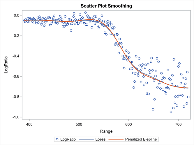
Both scatter plot smoothing techniques show a significant nonlinear structure between Range and LogRatio that cannot be easily modeled by ordinary polynomials. You can also use the GAMPL procedure to perform scatter plot smoothing
on this data set, as in the following statements:
proc gampl data=Lidar seed=12345;
   model LogRatio = spline(Range/details);
   output out=LidarOut pred=p;
run;
The “Specifications for Spline(Range)” table in Output 42.1.2 displays the specifications for constructing the spline term for Range. The maximum degrees of freedom is 10, which sets the upper limit of effective degrees of freedom for the spline term to
be 9 after one degree of freedom is absorbed in the intercept. The order of the derivative in the penalty is 2, which means
the unpenalized portion of the spline term involves polynomials with degrees up to 2.
Output 42.1.2: Spline Specification
The “Fit Statistics” table in Output 42.1.3 shows the summary statistics for the fitted model.
Output 42.1.3: Fit Statistics
| Fit Statistics | |
|---|---|
| Penalized Log Likelihood | 251.44124 |
| Roughness Penalty | 0.00000426 |
| Effective Degrees of Freedom | 9.99988 |
| Effective Degrees of Freedom for Error | 211.00000 |
| AIC (smaller is better) | -482.88271 |
| AICC (smaller is better) | -481.83512 |
| BIC (smaller is better) | -448.90148 |
| GCV (smaller is better) | 0.00654 |
The “Estimates for Smoothing Components” table in Output 42.1.4 shows that the effective degrees of freedom for the spline term of Range is approximately 8 after the GCV criterion is optimized with respect to the smoothing parameter. The roughness penalty is
small, suggesting that there is an important contribution from the penalized part of thin-plate regression splines beyond
nonpenalized polynomials.
Output 42.1.4: Estimates for Smoothing Components
Because the optimal model is obtained by searching in a functional space that is constrained by the maximum degrees of freedom for a spline term, you might wonder whether PROC GAMPL produces a much different model if you increase the value. The following statements fit another model in which the maximum degrees of freedom is increased to 20:
proc gampl data=Lidar seed=12345;
   model LogRatio = spline(Range/maxdf=20);
   output out=LidarOut2 pred=p2;
run;
Output 42.1.5 displays fit summary statistics for the second model. The model fit statistics from the second model are very close to the ones from the first model, indicating that the second model is not much different from the first model.
Output 42.1.5: Fit Statistics
| Scatter Plot Smoothing |
| Fit Statistics | |
|---|---|
| Penalized Log Likelihood | 250.95136 |
| Roughness Penalty | 0.06254 |
| Effective Degrees of Freedom | 10.04384 |
| Effective Degrees of Freedom for Error | 209.03211 |
| AIC (smaller is better) | -481.87757 |
| AICC (smaller is better) | -480.82094 |
| BIC (smaller is better) | -447.74696 |
| GCV (smaller is better) | 0.00657 |
Output 42.1.6 shows that the effective degrees of freedom for the spline term of Range is slightly larger than 8, which is understandable because increasing the maximum degrees of freedom expands the functional
space for model searching. Functions in the expanded space can provide a better fit to the data, but they are also penalized
more because the roughness penalty value for the second model is much larger than the one for the first model. This suggests
that functions in the expanded space do not help much, given the nonlinear relationship between Range and LogRatio.
Output 42.1.6: Estimates for Smoothing Components
The two fitted models are all based on thin-plate regression splines, in which polynomials that have degrees higher than 2 are penalized. You might wonder whether allowing higher-order polynomials yields a much different model. The following statements fit a third spline model by penalizing polynomials that have degrees higher than 3:
proc gampl data=Lidar seed=12345;
   model LogRatio = spline(Range/m=3);
   output out=LidarOut3 pred=p3;
run;
The fit summary statistics shown in Output 42.1.7 are close to the ones from the previous two models, albeit slightly smaller.
Output 42.1.7: Fit Statistics
| Scatter Plot Smoothing |
| Fit Statistics | |
|---|---|
| Penalized Log Likelihood | 249.79779 |
| Roughness Penalty | 9.440383E-9 |
| Effective Degrees of Freedom | 10.00000 |
| Effective Degrees of Freedom for Error | 211.00000 |
| AIC (smaller is better) | -479.59559 |
| AICC (smaller is better) | -478.54797 |
| BIC (smaller is better) | -445.61397 |
| GCV (smaller is better) | 0.00664 |
As shown in Output 42.1.8, the effective degrees of freedom for the spline term where polynomials with degrees less than 4 are allowed without penalization is 8. The roughness penalty is quite small compared to the previous two fits. This also suggests that there are important contributions from the penalized part of the thin-plate regression splines even after the nonpenalized polynomials are raised to order 3.
Output 42.1.8: Estimates for Smoothing Components
The following statements use the DATA step to merge the predictions from the three scatter plot smoothing fits by PROC GAMPL and use the SGPLOT procedure to visualize them:
data LidarPred;
   merge Lidar LidarOut LidarOut2 LidarOut3;
run;

proc sgplot data=LidarPred;
   scatter x=Range y=LogRatio / markerattrs=GraphData1(size=7);
   series  x=Range y=p        / lineattrs  =GraphData2(thickness=2)
                                legendlabel="Spline 1";
   series  x=Range y=p2       / lineattrs  =GraphData3(thickness=2)
                                legendlabel="Spline 2";
   series  x=Range y=p3       / lineattrs  =GraphData4(thickness=2)
                                legendlabel="Spline 3";
run;
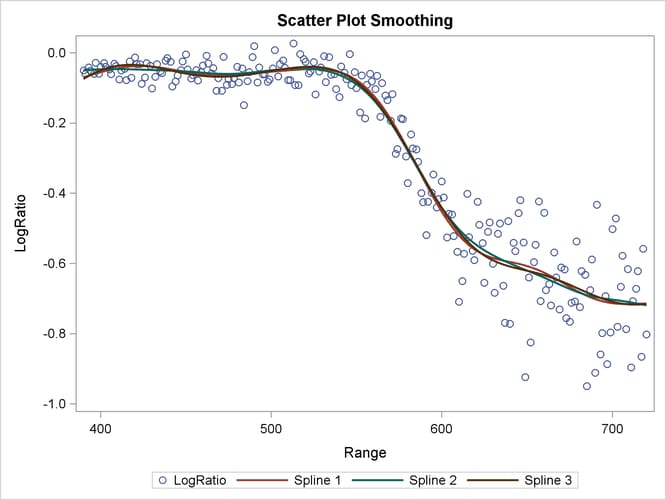
Output 42.1.9 displays the scatter plot smoothing fits by PROC GAMPL under three different spline specifications.
Output 42.1.9: Scatter Plot Smoothing