The GAMPL Procedure
-
Overview

- Getting Started
-
Syntax
-
DetailsMissing ValuesThin-Plate Regression SplinesGeneralized Additive ModelsModel Evaluation CriteriaFitting AlgorithmsDegrees of FreedomModel InferenceDispersion ParameterTests for Smoothing ComponentsComputational Method: MultithreadingChoosing an Optimization TechniqueDisplayed OutputODS Table NamesODS Graphics
-
Examples
- References
Tests for Smoothing Components
The GAMPL procedure performs a smoothing component test on the null hypotheses  for the jth component. In contrast to the analysis of deviance that is used in PROC GAM (which tests existence of nonlinearity for
each smoothing component), the smoothing component test used in PROC GAMPL tests for the existence of a contribution for each
smoothing component.
for the jth component. In contrast to the analysis of deviance that is used in PROC GAM (which tests existence of nonlinearity for
each smoothing component), the smoothing component test used in PROC GAMPL tests for the existence of a contribution for each
smoothing component.
The hypothesis test is based on the Wald statistic. Define  as the matrix of all zeros except for columns that correspond to basis expansions of the jth spline term. Then the column vector of predictions is
  , and the covariance matrix for the predictions is
  . The Wald statistic for testing is
![\[ T_ r = \hat{\mb{f}}_ j’\bV _ j^{r-}\hat{\mb{f}}_ j = \hat{\bbeta }’\bX _ j’(\bX _ j\bV _{\bbeta }\bX _ j’)^{r-}\bX _ j\hat{\bbeta } \]](images/statug_hpgam0210.png)
where  is the rank-r pseudo-inverse of
  . If
. If  is the Cholesky root for
  such that
  , then the test statistic can be written as
![\[ T_ r = \hat{\bbeta }’\bR _ j’(\bR _ j\bV _{\bbeta }\bR _ j’)^{r-}\bR _ j\hat{\bbeta } \]](images/statug_hpgam0215.png)
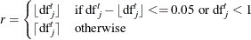
Wood (2012) proposes using the  degrees of freedom for test (which is defined in the section Degrees of Freedom) as the rank r. Because spline terms in fitted models often have noninteger degrees of freedom, the GAMPL procedure uses a rounded value
of as the rank:
degrees of freedom for test (which is defined in the section Degrees of Freedom) as the rank r. Because spline terms in fitted models often have noninteger degrees of freedom, the GAMPL procedure uses a rounded value
of as the rank:
Let K be a symmetric and nonnegative definite matrix, and let its eigenvalues be sorted as  ; then the rank-r pseudo-inverse of K is formed by
![\[ K^{r-} = U_ k\begin{bmatrix} d_1^{-1} & & \\ & \ddots & \\ & & d_ r^{-1} \end{bmatrix}U_ k’ \]](images/statug_hpgam0219.png)
where  are formed by columns of eigenvectors that correspond to the r eigenvalues.
Under the null hypothesis, the Wald statistic  approximately follows the chi-square distribution
  . For an observed test statistic
  , the p-value for rejecting the null hypothesis is computed as
  if the dispersion parameter is constant, or
  with
with  error degrees of freedom if the dispersion parameter is estimated.
Be cautious when you interpret the results of the smoothing component test because p-values are computed by approximation and the test does not take the smoothing parameter selection process into account.