The CALIS Procedure
-
Overview

-
Getting Started
-
SyntaxClasses of Statements in PROC CALISSingle-Group Analysis SyntaxMultiple-Group Multiple-Model Analysis SyntaxPROC CALIS StatementBOUNDS StatementBY StatementCOSAN StatementCOV StatementDETERM StatementEFFPART StatementFACTOR StatementFITINDEX StatementFREQ StatementGROUP StatementLINCON StatementLINEQS StatementLISMOD StatementLMTESTS StatementMATRIX StatementMEAN StatementMODEL StatementMSTRUCT StatementNLINCON StatementNLOPTIONS StatementOUTFILES StatementPARAMETERS StatementPARTIAL StatementPATH StatementPATHDIAGRAM StatementPCOV StatementPVAR StatementRAM StatementREFMODEL StatementRENAMEPARM StatementSAS Programming StatementsSIMTESTS StatementSTD StatementSTRUCTEQ StatementTESTFUNC StatementVAR StatementVARIANCE StatementVARNAMES StatementWEIGHT Statement
-
DetailsInput Data SetsOutput Data SetsDefault Analysis Type and Default ParameterizationThe COSAN ModelThe FACTOR ModelThe LINEQS ModelThe LISMOD Model and SubmodelsThe MSTRUCT ModelThe PATH ModelThe RAM ModelNaming Variables and ParametersSetting Constraints on ParametersAutomatic Variable SelectionPath Diagrams: Layout Algorithms, Default Settings, and CustomizationEstimation CriteriaRelationships among Estimation CriteriaGradient, Hessian, Information Matrix, and Approximate Standard ErrorsCounting the Degrees of FreedomAssessment of FitCase-Level Residuals, Outliers, Leverage Observations, and Residual DiagnosticsTotal, Direct, and Indirect EffectsStandardized SolutionsModification IndicesMissing Values and the Analysis of Missing PatternsMeasures of Multivariate KurtosisInitial EstimatesUse of Optimization TechniquesComputational ProblemsDisplayed OutputODS Table NamesODS Graphics
-
ExamplesEstimating Covariances and CorrelationsEstimating Covariances and Means SimultaneouslyTesting Uncorrelatedness of VariablesTesting Covariance PatternsTesting Some Standard Covariance Pattern HypothesesLinear Regression ModelMultivariate Regression ModelsMeasurement Error ModelsTesting Specific Measurement Error ModelsMeasurement Error Models with Multiple PredictorsMeasurement Error Models Specified As Linear EquationsConfirmatory Factor ModelsConfirmatory Factor Models: Some VariationsResidual Diagnostics and Robust EstimationThe Full Information Maximum Likelihood MethodComparing the ML and FIML EstimationPath Analysis: Stability of AlienationSimultaneous Equations with Mean Structures and Reciprocal PathsFitting Direct Covariance StructuresConfirmatory Factor Analysis: Cognitive AbilitiesTesting Equality of Two Covariance Matrices Using a Multiple-Group AnalysisTesting Equality of Covariance and Mean Matrices between Independent GroupsIllustrating Various General Modeling LanguagesTesting Competing Path Models for the Career Aspiration DataFitting a Latent Growth Curve ModelHigher-Order and Hierarchical Factor ModelsLinear Relations among Factor LoadingsMultiple-Group Model for Purchasing BehaviorFitting the RAM and EQS Models by the COSAN Modeling LanguageSecond-Order Confirmatory Factor AnalysisLinear Relations among Factor Loadings: COSAN Model SpecificationOrdinal Relations among Factor LoadingsLongitudinal Factor Analysis
- References
This example illustrates case-level residual diagnostics and robust estimation with PROC CALIS. The data set is available in Mardia, Kent, and Bibby (1979). It contains 88 responses on five subjects: mechanics, vector, algebra, analysis, and statistics. Yuan and Hayashi (2010) use the same data set to illustrate the uses of residual diagnostics in the context of robust estimation. Inspired by their illustrations, this example mirrors their one-factor model, with some modifications.
The following DATA step specifies and inputs five observed variables for the data set mardia:
data mardia;
   input mechanics vector algebra analysis statistics;
   datalines;
77.000     82.000     67.000     67.000     81.000
63.000     78.000     80.000     70.000     81.000
75.000     73.000     71.000     66.000     81.000
  .          .          .          .          .
  .          .          .          .          .
     { More Data }
  .          .          .          .          .
  .          .          .          .          .
  .          .          .          .          .
  .          .          .          .          .
;
You specify a one-factor model for the five variables by using the following statements:
ods graphics on;

proc calis data=mardia residual plots=caseresid;
   path
      fact1 ===>  mechanics vector algebra analysis statistics = 1. ;
run;

ods graphics off;
In the PATH statement, all observed variables are indicators of the latent factor fact1. The first factor loading for mechanics is fixed at 1 for identification of the latent variable scale, while the remaining four loadings are free parameters in the
model. The RESIDUAL option that is specified in the PROC CALIS statement requests residual analysis. Because raw data are
input, case-level residual analysis is done. To request all the available ODS Graphics output for case-level residual diagnostics,
you specify the PLOTS=CASERESID option. To enable ODS Graphics, you specify the ODS GRAPHICS ON statement before running the
CALIS procedure.
Output 29.14.1 shows some of the fit statistics of the one-factor model. The model fit chi-square is 8.9782 (df = 5, p = 0.1099). Therefore, you fail to reject the one-factor model for the data. The SRMR is 0.0411, which shows a good fit. But the RMSEA is 0.0956, which does not show that the one-factor model is a very good approximating model for the data. Output 29.14.2 shows the loading estimates. All are statistically significant.
Output 29.14.2: Estimates of Loadings
| PATH List | |||||||
|---|---|---|---|---|---|---|---|
| Path | Parameter | Estimate | Standard Error |
t Value | Pr > |t| | ||
| fact1 | ===> | mechanics | 1.00000 | ||||
| fact1 | ===> | vector | _Parm1 | 0.83770 | 0.16598 | 5.0469 | <.0001 |
| fact1 | ===> | algebra | _Parm2 | 0.93064 | 0.15369 | 6.0552 | <.0001 |
| fact1 | ===> | analysis | _Parm3 | 1.09480 | 0.19611 | 5.5826 | <.0001 |
| fact1 | ===> | statistics | _Parm4 | 1.19229 | 0.22309 | 5.3444 | <.0001 |
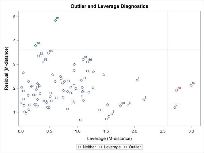
Output 29.14.3 shows the classifications of outlier and leverage observations in a two-dimensional space. Four regions are clearly shown.
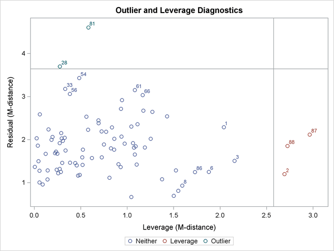
The upper and the lower regions are separated by a horizontal line that represents the criterion for outlier detection. This
criterion is set by a certain ![]() -level that has a probability meaning. Loosely speaking, if the model is true and the distribution of the residuals is multivariate
normal, you would expect that about
-level that has a probability meaning. Loosely speaking, if the model is true and the distribution of the residuals is multivariate
normal, you would expect that about ![]() of observations will have their residual M-distances above the criterion. The larger the
of observations will have their residual M-distances above the criterion. The larger the ![]() value, the more liberal the outlier detection criterion. This
value, the more liberal the outlier detection criterion. This ![]() -level is set to 0.01 by default. You can change this default by using the ALPHAOUT=
option.
-level is set to 0.01 by default. You can change this default by using the ALPHAOUT=
option.
Notice that all residuals and the criterion are measured in terms of M-distances. Hence, these measures are always positive. Output 29.14.3 classifies observations 81 and 28 as outliers (in the residual dimension). In addition to these two outlying observations, PROC CALIS also labels the next five observations with the largest residual M-distances. Output 29.14.3 shows that observations 33, 54, 56, 61, and 66 are the closest to being labeled as outliers.
The right and left regions are separated by a vertical line that represents the criterion for leverage observations. Again,
this criterion is set by a certain ![]() -level that has a probability meaning. If the model is true and the distribution of the predictor variables (in this case,
the factor variable
-level that has a probability meaning. If the model is true and the distribution of the predictor variables (in this case,
the factor variable fact1) is multivariate normal, you would expect that about ![]() of observations will have their leverage M-distances above the criterion. The larger the
of observations will have their leverage M-distances above the criterion. The larger the ![]() value, the more liberal the leverage observation detection criterion. This
value, the more liberal the leverage observation detection criterion. This ![]() -level is also set to 0.01 by default. You can change this default by using the ALPHALEV=
option.
-level is also set to 0.01 by default. You can change this default by using the ALPHALEV=
option.
Output 29.14.3 classifies observations 2, 87, and 88 as leverage points or observations. In addition to these three observations, PROC CALIS also labels the next five observations with the largest leverage M-distances. Output 29.14.3 shows that observations 1, 3, 6, 8, and 86 are the closest to being labeled as leverage observations.
The lower left region in Output 29.14.3 contains observations that are neither outliers nor leverage observations. This region contains the majority of the observations. The upper right region in Output 29.14.3 contains observations that are classified as both outliers and leverage observations. For the current model, no observations are classified as such.
To supplement the graphical depiction of outliers and leverage observations, PROC CALIS shows two tables that contain more numerical information. Output 29.14.4 shows the seven observations that have the largest residual M-distances. The table reflects the outlier classification in Output 29.14.3 numerically. Two outliers are flagged in the table. However, none of the seven observations are leverage observations. Output 29.14.5 shows the eight observations that have the largest leverage M-distances. Again, this table reflects the classification of leverage observations in Output 29.14.3 numerically. Three leverage observations are flagged, but none of these observations are residual outliers at the same time.
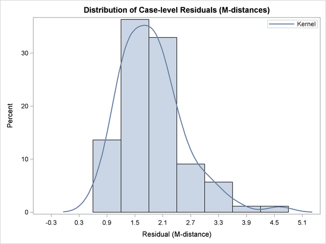
Output 29.14.6 shows the histogram and its kernel density function of the residual M-distances. Theoretically, the density should look like
a ![]() -distribution (that is, the distribution of the square root of the corresponding
-distribution (that is, the distribution of the square root of the corresponding ![]() variate). While this histogram provides an overall impression of the empirical distribution of the residual M-distances,
it is not very useful in diagnosing the observations that do not conform to the theoretical distribution of the residual M-distances.
To this end, Output 29.14.7 and Output 29.14.8 are more useful.
variate). While this histogram provides an overall impression of the empirical distribution of the residual M-distances,
it is not very useful in diagnosing the observations that do not conform to the theoretical distribution of the residual M-distances.
To this end, Output 29.14.7 and Output 29.14.8 are more useful.
Output 29.14.7 shows the so-called Q-Q plot for the residual M-distances. The Y coordinates represent the observed quantiles, and the X
coordinates represent the theoretical quantiles. Output 29.14.8 shows the so-called P-P plots for the residual M-distances. The Y coordinates represent the observed percentiles, and the
X coordinates represent the theoretical percentiles. If the observed residual M-distances distribute exactly like the theoretical
![]() -distribution, all observations should lie on the straight lines with a slope of 1 in both plots. In Output 29.14.7 and Output 29.14.8, observations with the largest departures from the straight lines are labeled.
-distribution, all observations should lie on the straight lines with a slope of 1 in both plots. In Output 29.14.7 and Output 29.14.8, observations with the largest departures from the straight lines are labeled.
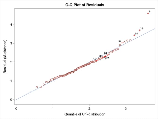
In terms of quantiles, the Q-Q plot in Output 29.14.7 shows that observations 81, 28, and 54 have the largest departures from the theoretical distribution for the residual M-distances. Notice that observations 81 and 28 were also identified as outliers previously.
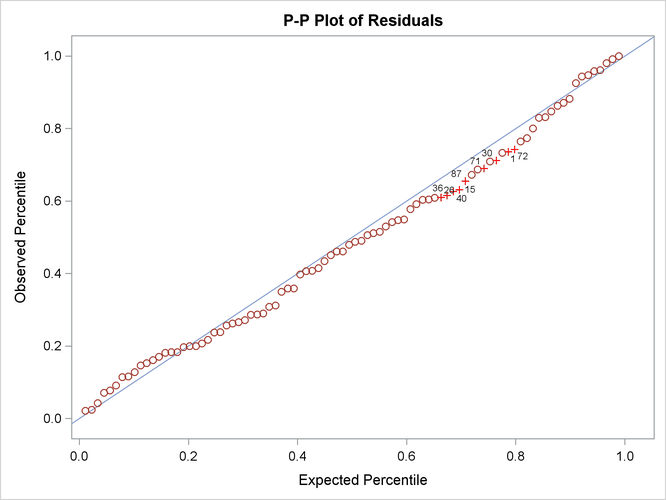
In terms of percentiles, the P-P plot in Output 29.14.8 shows that several observations in the middle of the distribution have the largest departures from the theoretical distribution. However, it is not clear from the plot which observations have the largest departures.
To supplement the Q-Q and the P-P plots with numerical information, PROC CALIS outputs the table in Output 29.14.9, which shows the observations with the largest departures from the theoretical residual M-distance distribution in terms
of quantiles and percentiles. The observations in the table are arranged by their percentile regions. Approximately 10![]() of the observations with the largest departures in terms of quantile and in terms of percentile, respectively, are shown
in this table. However, the final percentage of observations shown in the table might not add up to 20
of the observations with the largest departures in terms of quantile and in terms of percentile, respectively, are shown
in this table. However, the final percentage of observations shown in the table might not add up to 20![]() , because some observations could have large departures in terms of both quantile and percentile. Output 29.14.9 shows that observations 1, 15, 30, and 72 are this kind of observation. However, none of these are residual outliers.
, because some observations could have large departures in terms of both quantile and percentile. Output 29.14.9 shows that observations 1, 15, 30, and 72 are this kind of observation. However, none of these are residual outliers.
Output 29.14.9: Largest Departures from the Theoretical Residual Distribution
| Largest Departures From the Theoretical Residual Distribution |
|||
|---|---|---|---|
| Percentile Region |
Case Number |
Quantile Deviation |
Percentile Deviation |
| (.65,.90) | 26 | -0.05302 | |
| 36 | -0.05836 | ||
| 40 | -0.05863 | ||
| 15 | -0.13087 | -0.06509 | |
| 87 | -0.05257 | ||
| 71 | -0.05145 | ||
| 30 | -0.11973 | -0.05198 | |
| 1 | -0.12344 | -0.05065 | |
| 72 | -0.13739 | -0.05498 | |
| 64 | -0.12550 | ||
| (.90,.95) | 66 | 0.13803 | |
| >.95 | 54 | 0.20039 | |
| 28 | 0.32398 | ||
| 81 | 0.99843 | ||
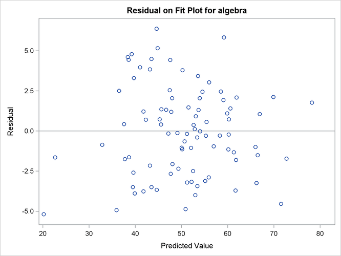
Output 29.14.10 shows the residual on fit plot for the variable algebra. Notice that unlike the preceding residual diagnostic plots where the M-distances (nonnegative) for residuals are plotted,
the residuals (which can be positive or negative) themselves are plotted against the predicted values for algebra in the current residual on fit (or residual on predicted) plot. If the linear relationship as described by the one-factor
model is reasonable, then the residuals should show no systematic trend with the predicted values. That is, the residuals
should be randomly scattered around the plot in the range of the predicted values. The pattern of residuals in Output 29.14.10 looks sufficiently "random," and therefore it gives support to the prescribed linear relationship between the variable algebra and the factor fact1. PROC CALIS also outputs the residual on fit plots for other dependent observed variables. To conserve space, they are not
shown here. You can also control the amount of graphical output by specifying the desirable set of dependent observed variables
for the residual on fit plots. For example, the following requests the residual on fit plots for the variables mechanics and analysis only, even though there are five dependent observed variables in the model:
PLOTS=RESBYPRED(VAR=mechanics analysis)
See the PLOTS= option for details.
Usually, the outlier detection process in residual diagnostics implies some treatments after their detections. For example, in the preceding analysis, observations 28 and 81 were detected as outliers. You would naturally think that the next step is to do an additional model fitting with these two outlying observations removed. While this thinking is intuitively appealing, the outlier issues are usually more complicated than can be resolved by such a "pick-and-remove" strategy. One issue is the so-called masking effect of outliers. In the preceding analysis, outliers are detected based on a criterion that is a function of the chosen criterion level (for example, the ALPHAOUT= value set by the researcher) and the parameter estimates. However, because the outliers have contributed to the estimation of the parameters, you might wonder whether the outlier detection process has been contaminated by the outliers themselves. If such a masking effect is present and an additional analysis is done after employing the pick-and-remove strategy for the outliers, you would be likely to discover more outliers. As a result, you might wonder whether the outlier removal process should be carried out indefinitely.
Robust estimation provides an alternative way to resolve the issue of masking effect. In robust estimation, outlying observations are downweighted simultaneously with the estimation. Iterative steps are used to reweight the observations according to the updated parameter estimates. Hence, with robust estimation you do not need to make a decision about removing outliers because they are already downweighted during the estimation. The issue of masking effect is avoided.
PROC CALIS provides two major methods of robust estimation—direct and two-stage. This section illustrates the direct robust estimation method, in which the model is estimated simultaneously with the (re)weighting of the observations. The next section illustrates the two-stage estimation method, in which the robust mean and covariance matrices obtained in the first stage are analyzed by the maximum likelihood (ML) estimation in the second stage. Both methods are based on the methodology proposed by Yuan and Zhong (2008) and Yuan and Hayashi (2010).
The following statements request direct robust estimation of the model for the mardia data set:
ods graphics on;

proc calis data=mardia residual robust plots=caseresid pcorr;
   path
      fact1 ===>  mechanics vector algebra analysis statistics = 1. ;
run;

ods graphics off;
The ROBUST option invokes the direct robust estimation method. The direct robust method reweights the observations according to the magnitudes of the residuals during iterative steps. For this reason, you can also specify ROBUST=RES to signify direct robust estimation with residual (M-distance) weighting. Following Yuan and Hayashi (2010), there are two variants of the direct robust estimation, One treats the disturbances (that is, error terms for endogenous latent factors) as factors to estimate (see the ROBUST= RES(F) option), and the other treats the disturbances as true error terms (see the ROBUST= RES(E) option). See the ROBUST= option and the section Robust Estimation for details. These variants would not make any difference for the current one-factor model estimation, and the ROBUST option that is used in the specification is the same as ROBUST=RES(E).
You also request case-level residual analysis by using the RESIDUAL option, even though the intention now is to identify rather than to remove the outliers.
Output 29.14.11 shows the fit summary of the direct robust estimation. The model fit chi-square is 6.0031 (df = 5, p = 0.3059). Again, you fail to reject the one-factor model for the data. Unlike the regular ML estimation in the preceding analysis, both SRMR (0.0321) and RMSEA (0.0480) show good model fit. This result can be attributed to the downweighting of the outlying observations in the direct robust estimation. Output 29.14.12 shows that all loading estimates are statistically significant.
Output 29.14.12: Estimates of Loadings with Direct Robust Estimation
| PATH List | |||||||
|---|---|---|---|---|---|---|---|
| Path | Parameter | Estimate | Standard Error |
t Value | Pr > |t| | ||
| fact1 | ===> | mechanics | 1.00000 | ||||
| fact1 | ===> | vector | _Parm1 | 0.83279 | 0.15680 | 5.3111 | <.0001 |
| fact1 | ===> | algebra | _Parm2 | 0.92854 | 0.14763 | 6.2895 | <.0001 |
| fact1 | ===> | analysis | _Parm3 | 1.08665 | 0.18855 | 5.7632 | <.0001 |
| fact1 | ===> | statistics | _Parm4 | 1.18799 | 0.21487 | 5.5289 | <.0001 |
Output 29.14.13 shows the outlier and leverage classifications by the direct robust estimation. This plot has a similar pattern to the one obtained from the preceding regular ML estimation (see Output 29.14.3). Both plots show that observations 28 and 81 are the only outliers. Thus, the results from the direct robust estimation eliminate the concern of the masking effect.
As a by-product of the direct robust estimation, robust (unstructured) covariance and mean matrices are computed with the
PCORR
option. Output 29.14.14 shows the robust covariance and mean matrices obtained for the current direct robust estimation for the mardia data set. These matrices are essentially computed by the usual formulas for covariance and mean matrices, but with weights
obtained from the final estimates of the direct robust estimation of the model. For the current analysis, outlying observations
(28 and 81) receive weights of less than 1 whereas all other observations receive weights of 1 in the computation.
Output 29.14.14: Robust Covariance and Mean Matrices with Direct Robust Estimation
| Robust Covariance Matrix | |||||
|---|---|---|---|---|---|
| mechanics | vector | algebra | analysis | statistics | |
| mechanics | 299.05121 | 118.73107 | 104.04139 | 111.35028 | 122.12239 |
| vector | 118.73107 | 162.60829 | 86.88667 | 97.18075 | 102.10393 |
| algebra | 104.04139 | 86.88667 | 114.69031 | 113.43289 | 124.09414 |
| analysis | 111.35028 | 97.18075 | 113.43289 | 220.34769 | 156.62425 |
| statistics | 122.12239 | 102.10393 | 124.09414 | 156.62425 | 296.42019 |
In addition to the direct robust estimation method, PROC CALIS implements another robust estimation method for structural equation models. The two-stage robust estimation method estimates the robust means and covariance matrices in the first stage. It then fits the model to the robust mean and covariance matrix by using the ML method in the second stage. During the first stage, the robust method downweights the outlying observations in all variable dimensions. The robust properties are then propagated to the second stage of estimation.
In PROC CALIS, you can use the ROBUST=SAT option to invoke the two-stage robust estimation method, as shown in the following
statements for fitting the one-factor model to the mardia data set:
proc calis data=mardia robust=sat pcorr;
   path
      fact1 ===>  mechanics vector algebra analysis statistics = 1. ;
run;
With the PCORR option, the (unstructured) robust mean and covariance matrices are displayed in Output 29.14.15. Although the robust covariance and mean matrices obtained here are numerically similar to those obtained from the direct robust estimation (see Output 29.14.14), they are obtained with totally different methods. The robust mean and covariance matrices in the direct robust estimation are the by-products of the model estimation, while the robust mean and covariance matrices in the two-stage robust estimation are the initial inputs for model estimation.
Output 29.14.15: Robust Covariance and Mean Matrices with Two-Stage Robust Estimation
| Robust Covariance Matrix | |||||
|---|---|---|---|---|---|
| mechanics | vector | algebra | analysis | statistics | |
| mechanics | 298.83513 | 119.28292 | 99.65134 | 105.47098 | 116.68242 |
| vector | 119.28292 | 165.11323 | 84.25310 | 94.28855 | 98.70260 |
| algebra | 99.65134 | 84.25310 | 110.93012 | 110.46759 | 121.18480 |
| analysis | 105.47098 | 94.28855 | 110.46759 | 219.56424 | 155.24377 |
| statistics | 116.68242 | 98.70260 | 121.18480 | 155.24377 | 298.80146 |
Output 29.14.16 shows the fit summary of the two-stage robust estimation. The model fit chi-square is 7.2941 (df = 5, p = 0.1997). As in direct robust estimation, you fail to reject the one-factor model for the data. Unlike the case with direct robust estimation, only SRMR (0.0366) shows a good model fit. RMSEA is 0.0726 and is not very close to a good model fit.
Output 29.14.16 shows the estimates of loadings with the two-stage robust estimation. All the estimates are statistically significant. All the numerical results are similar to that of the direct robust estimation in Output 29.14.12.
Output 29.14.17: Estimates of Loadings with Two-Stage Robust Estimation
| PATH List | |||||||
|---|---|---|---|---|---|---|---|
| Path | Parameter | Estimate | Standard Error |
t Value | Pr > |t| | ||
| fact1 | ===> | mechanics | 1.00000 | ||||
| fact1 | ===> | vector | _Parm1 | 0.84322 | 0.16538 | 5.0986 | <.0001 |
| fact1 | ===> | algebra | _Parm2 | 0.93683 | 0.15485 | 6.0500 | <.0001 |
| fact1 | ===> | analysis | _Parm3 | 1.10397 | 0.19849 | 5.5617 | <.0001 |
| fact1 | ===> | statistics | _Parm4 | 1.21080 | 0.22686 | 5.3371 | <.0001 |
The outlier and leverage observation detection in two-stage robust estimation is essentially the same method as that in direct robust estimation. Therefore, the corresponding results for the two-stage robust estimation are not shown here. See the section Residual Diagnostics with Robust Estimation for details about case-level residual analysis with robust estimation.