The CALIS Procedure
-
Overview

-
Getting Started
-
SyntaxClasses of Statements in PROC CALISSingle-Group Analysis SyntaxMultiple-Group Multiple-Model Analysis SyntaxPROC CALIS StatementBOUNDS StatementBY StatementCOSAN StatementCOV StatementDETERM StatementEFFPART StatementFACTOR StatementFITINDEX StatementFREQ StatementGROUP StatementLINCON StatementLINEQS StatementLISMOD StatementLMTESTS StatementMATRIX StatementMEAN StatementMODEL StatementMSTRUCT StatementNLINCON StatementNLOPTIONS StatementOUTFILES StatementPARAMETERS StatementPARTIAL StatementPATH StatementPATHDIAGRAM StatementPCOV StatementPVAR StatementRAM StatementREFMODEL StatementRENAMEPARM StatementSAS Programming StatementsSIMTESTS StatementSTD StatementSTRUCTEQ StatementTESTFUNC StatementVAR StatementVARIANCE StatementVARNAMES StatementWEIGHT Statement
-
DetailsInput Data SetsOutput Data SetsDefault Analysis Type and Default ParameterizationThe COSAN ModelThe FACTOR ModelThe LINEQS ModelThe LISMOD Model and SubmodelsThe MSTRUCT ModelThe PATH ModelThe RAM ModelNaming Variables and ParametersSetting Constraints on ParametersAutomatic Variable SelectionPath Diagrams: Layout Algorithms, Default Settings, and CustomizationEstimation CriteriaRelationships among Estimation CriteriaGradient, Hessian, Information Matrix, and Approximate Standard ErrorsCounting the Degrees of FreedomAssessment of FitCase-Level Residuals, Outliers, Leverage Observations, and Residual DiagnosticsTotal, Direct, and Indirect EffectsStandardized SolutionsModification IndicesMissing Values and the Analysis of Missing PatternsMeasures of Multivariate KurtosisInitial EstimatesUse of Optimization TechniquesComputational ProblemsDisplayed OutputODS Table NamesODS Graphics
-
ExamplesEstimating Covariances and CorrelationsEstimating Covariances and Means SimultaneouslyTesting Uncorrelatedness of VariablesTesting Covariance PatternsTesting Some Standard Covariance Pattern HypothesesLinear Regression ModelMultivariate Regression ModelsMeasurement Error ModelsTesting Specific Measurement Error ModelsMeasurement Error Models with Multiple PredictorsMeasurement Error Models Specified As Linear EquationsConfirmatory Factor ModelsConfirmatory Factor Models: Some VariationsResidual Diagnostics and Robust EstimationThe Full Information Maximum Likelihood MethodComparing the ML and FIML EstimationPath Analysis: Stability of AlienationSimultaneous Equations with Mean Structures and Reciprocal PathsFitting Direct Covariance StructuresConfirmatory Factor Analysis: Cognitive AbilitiesTesting Equality of Two Covariance Matrices Using a Multiple-Group AnalysisTesting Equality of Covariance and Mean Matrices between Independent GroupsIllustrating Various General Modeling LanguagesTesting Competing Path Models for the Career Aspiration DataFitting a Latent Growth Curve ModelHigher-Order and Hierarchical Factor ModelsLinear Relations among Factor LoadingsMultiple-Group Model for Purchasing BehaviorFitting the RAM and EQS Models by the COSAN Modeling LanguageSecond-Order Confirmatory Factor AnalysisLinear Relations among Factor Loadings: COSAN Model SpecificationOrdinal Relations among Factor LoadingsLongitudinal Factor Analysis
- References
The following seven estimation methods are available in PROC CALIS:
-
unweighted least squares (ULS)
-
full information maximum likelihood (FIML)
-
generalized least squares (GLS)
-
normal-theory maximum likelihood (ML)
-
weighted least squares (WLS, ADF)
-
diagonally weighted least squares (DWLS)
-
robust estimation (ROBUST) under the normal theory (ML)
Default weight matrices ![]() are computed for GLS, WLS, and DWLS estimation. You can also provide your own weight matrices by using an INWGT=
data set. The weight matrices in these estimation methods provide weights for the moment matrices. In contrast, weights that
are applied to individual observations are computed in robust estimation. These observation weights are updated during iteration
steps of robust estimation. The ULS, GLS, ML, WLS, ADF, and DWLS methods can analyze sample moment matrices as well as raw
data, while the FIML and robust methods must analyze raw data.
are computed for GLS, WLS, and DWLS estimation. You can also provide your own weight matrices by using an INWGT=
data set. The weight matrices in these estimation methods provide weights for the moment matrices. In contrast, weights that
are applied to individual observations are computed in robust estimation. These observation weights are updated during iteration
steps of robust estimation. The ULS, GLS, ML, WLS, ADF, and DWLS methods can analyze sample moment matrices as well as raw
data, while the FIML and robust methods must analyze raw data.
PROC CALIS does not implement all estimation methods in the field. As mentioned in the section Overview: CALIS Procedure, partial least squares (PLS) is not implemented. The PLS method is developed under less restrictive statistical assumptions. It circumvents some computational and theoretical problems encountered by the existing estimation methods in PROC CALIS; however, PLS estimates are less efficient in general. When the statistical assumptions of PROC CALIS are tenable (for example, large sample size, correct distributional assumptions, and so on), ML, GLS, or WLS methods yield better estimates than the PLS method. Note that there is a SAS/STAT procedure called PROC PLS that employs the partial least squares technique, but for a different class of models than those of PROC CALIS. For example, in a PROC CALIS model each latent variable is typically associated with only a subset of manifest variables (predictor or outcome variables). However, in PROC PLS latent variables are not prescribed with subsets of manifest variables. Rather, they are extracted from linear combinations of all manifest predictor variables. Therefore, for general path analysis with latent variables you should use PROC CALIS.
In each estimation method, the parameter vector is estimated iteratively by a nonlinear optimization algorithm that minimizes
a discrepancy function F, which is also known as the fit function in the literature. With p denoting the number of manifest variables, ![]() the sample
the sample ![]() covariance matrix for a sample with size N,
covariance matrix for a sample with size N, ![]() the
the ![]() vector of sample means,
vector of sample means, ![]() the fitted covariance matrix, and
the fitted covariance matrix, and ![]() the vector of fitted means, the discrepancy function for unweighted least squares (ULS) estimation is:
the vector of fitted means, the discrepancy function for unweighted least squares (ULS) estimation is:
The discrepancy function for generalized least squares estimation (GLS) is:
By default, ![]() is assumed so that
is assumed so that ![]() is the normal theory generalized least squares discrepancy function.
is the normal theory generalized least squares discrepancy function.
The discrepancy function for normal-theory maximum likelihood estimation (ML) is:
In each of the discrepancy functions, ![]() and
and ![]() are considered to be given and
are considered to be given and ![]() and
and ![]() are functions of model parameter vector
are functions of model parameter vector ![]() . That is:
. That is:
Estimating ![]() by using a particular estimation method amounts to choosing a vector
by using a particular estimation method amounts to choosing a vector ![]() that minimizes the corresponding discrepancy function F.
that minimizes the corresponding discrepancy function F.
When the mean structures are not modeled or when the mean model is saturated by parameters, the last term of each fit function vanishes. That is, they become:
If, instead of being a covariance matrix, ![]() is a correlation matrix in the discrepancy functions,
is a correlation matrix in the discrepancy functions, ![]() would naturally be interpreted as the fitted correlation matrix. Although whether
would naturally be interpreted as the fitted correlation matrix. Although whether ![]() is a covariance or correlation matrix makes no difference in minimizing the discrepancy functions, correlational analyses
that use these functions are problematic because of the following issues:
is a covariance or correlation matrix makes no difference in minimizing the discrepancy functions, correlational analyses
that use these functions are problematic because of the following issues:
-
The diagonal of the fitted correlation matrix
 might contain values other than ones, which violates the requirement of being a correlation matrix.
-
Whenever available, standard errors computed for correlation analysis in PROC CALIS are straightforward generalizations of those of covariance analysis. In very limited cases these standard errors are good approximations. However, in general they are not even asymptotically correct.
-
The model fit chi-square statistic for correlation analysis might not follow the theoretical distribution, thus making model fit testing difficult.
Despite these issues in correlation analysis, if your primary interest is to obtain the estimates in the correlation models, you might still find PROC CALIS results for correlation analysis useful.
The statistical techniques used in PROC CALIS are primarily developed for the analysis of covariance structures, and hence COVARIANCE is the default option. Depending on the nature of your research, you can add the mean structures in the analysis by specifying mean and intercept parameters in your models. However, you cannot analyze mean structures simultaneously with correlation structures (see the CORRELATION option) in PROC CALIS.
The full information maximum likelihood method (FIML) assumes multivariate normality of the data. Suppose that you analyze a model that contains p observed variables. The discrepancy function for FIML is
where ![]() is a data vector for observation j, and
is a data vector for observation j, and ![]() is a constant term (to be defined explicitly later) independent of the model parameters
is a constant term (to be defined explicitly later) independent of the model parameters ![]() . In the current formulation,
. In the current formulation, ![]() ’s are not required to have the same dimensions. For example,
’s are not required to have the same dimensions. For example, ![]() could be a complete vector with all p variables present while
could be a complete vector with all p variables present while ![]() is a
is a ![]() vector with one missing value that has been excluded from the original
vector with one missing value that has been excluded from the original ![]() data vector. As a consequence, subscript j is also used in
data vector. As a consequence, subscript j is also used in ![]() and
and ![]() to denote the submatrices that are extracted from the entire
to denote the submatrices that are extracted from the entire ![]() structured mean vector
structured mean vector ![]() (
(![]() ) and
) and ![]() covariance matrix
covariance matrix ![]() (
(![]() ). In other words, in the current formulation
). In other words, in the current formulation ![]() and
and ![]() do not mean that each observation is fitted by distinct mean and covariance structures (although theoretically it is possible
to formulate FIML in such a way). The notation simply signifies that the dimensions of
do not mean that each observation is fitted by distinct mean and covariance structures (although theoretically it is possible
to formulate FIML in such a way). The notation simply signifies that the dimensions of ![]() and of the associated mean and covariance structures could vary from observation to observation.
and of the associated mean and covariance structures could vary from observation to observation.
Let ![]() be the number of variables without missing values for observation j. Then
be the number of variables without missing values for observation j. Then ![]() denotes a
denotes a ![]() data vector,
data vector, ![]() denotes a
denotes a ![]() vector of means (structured with model parameters),
vector of means (structured with model parameters), ![]() is a
is a ![]() matrix for variances and covariances (also structured with model parameters), and
matrix for variances and covariances (also structured with model parameters), and ![]() is defined by the following formula, which is a constant term independent of model parameters:
is defined by the following formula, which is a constant term independent of model parameters:
As a general estimation method, the FIML method is based on the same statistical principle as the ordinary maximum likelihood
(ML) method for multivariate normal data—that is, both methods maximize the normal theory likelihood function given the data.
In fact, ![]() used in PROC CALIS is related to the log-likelihood function L by the following formula:
used in PROC CALIS is related to the log-likelihood function L by the following formula:
Because the FIML method can deal with observations with various levels of information available, it is primarily developed as an estimation method that could deal with data with random missing values. See the section Relationships among Estimation Criteria for more details about the relationship between FIML and ML methods.
Whenever you use the FIML method, the mean structures are automatically assumed in the analysis. This is due to fact that there is no closed-form formula to obtain the saturated mean vector in the FIML discrepancy function if missing values are present in the data. You can certainly provide explicit specification of the mean parameters in the model by specifying intercepts in the LINEQS statement or means and intercepts in the MEAN or MATRIX statement. However, usually you do not need to do the explicit specification if all you need to achieve is to saturate the mean structures with p parameters (that is, the same number as the number of observed variables in the model). With METHOD=FIML, PROC CALIS uses certain default parameterizations for the mean structures automatically. For example, all intercepts of endogenous observed variables and all means of exogenous observed variables are default parameters in the model, making the explicit specification of these mean structure parameters unnecessary.
Another important discrepancy function to consider is the weighted least squares (WLS) function. Let ![]() be a
be a ![]() vector containing all nonredundant elements in the sample covariance matrix
vector containing all nonredundant elements in the sample covariance matrix ![]() and sample mean vector
and sample mean vector ![]() , with
, with ![]() representing the vector of the
representing the vector of the ![]() lower triangle elements of the symmetric matrix
lower triangle elements of the symmetric matrix ![]() , stacking row by row. Similarly, let
, stacking row by row. Similarly, let ![]() be a
be a ![]() vector containing all nonredundant elements in the fitted covariance matrix
vector containing all nonredundant elements in the fitted covariance matrix ![]() and the fitted mean vector
and the fitted mean vector ![]() , with
, with ![]() representing the vector of the
representing the vector of the ![]() lower triangle elements of the symmetric matrix
lower triangle elements of the symmetric matrix ![]() .
.
The WLS discrepancy function is:
where ![]() is a positive definite symmetric weight matrix with
is a positive definite symmetric weight matrix with ![]() rows and columns. Because
rows and columns. Because ![]() is a function of model parameter vector
is a function of model parameter vector ![]() under the structural model, you can write the WLS function as:
under the structural model, you can write the WLS function as:
Suppose that ![]() converges to
converges to ![]() with increasing sample size, where
with increasing sample size, where ![]() and
and ![]() denote the population covariance matrix and mean vector, respectively. By default, the WLS weight matrix
denote the population covariance matrix and mean vector, respectively. By default, the WLS weight matrix ![]() in PROC CALIS is computed from the raw data as a consistent estimate of the asymptotic covariance matrix
in PROC CALIS is computed from the raw data as a consistent estimate of the asymptotic covariance matrix ![]() of
of ![]() , with
, with ![]() partitioned as
partitioned as
where ![]() denotes the
denotes the ![]() asymptotic covariance matrix for
asymptotic covariance matrix for ![]() ,
, ![]() denotes the
denotes the ![]() asymptotic covariance matrix for
asymptotic covariance matrix for ![]() , and
, and ![]() denotes the
denotes the ![]() asymptotic covariance matrix between
asymptotic covariance matrix between ![]() and
and ![]() .
.
To compute the default weight matrix ![]() as a consistent estimate of
as a consistent estimate of ![]() , define a similar partition of the weight matrix
, define a similar partition of the weight matrix ![]() as:
as:
Each of the submatrices in the partition can now be computed from the raw data. First, define the biased sample covariance for variables i and j as:
and the sample fourth-order central moment for variables i, j, k, and l as:
The submatrices in ![]() are computed by:
are computed by:
Assuming the existence of finite eighth-order moments, this default weight matrix ![]() is a consistent but biased estimator of the asymptotic covariance matrix
is a consistent but biased estimator of the asymptotic covariance matrix ![]() .
.
By using the ASYCOV=
option, you can use Browne’s unbiased estimator (Browne, 1984, formula (3.8)) of ![]() as:
as:
![\begin{eqnarray*} [\mb{W}_{ss}]_{ij,kl} & =& \frac{N(N-1)}{(N-2)(N-3)} (\mb{t}_{ij,kl} - \mb{t}_{ij}\mb{t}_{kl}) \\ & & - \frac{N}{(N-2)(N-3)} (\mb{t}_{ik} \mb{t}_{jl} + \mb{t}_{il} \mb{t}_{jk} - \frac{2}{N-1} \mb{t}_{ij} \mb{t}_{kl}) \end{eqnarray*}](images/statug_calis0509.png)
There is no guarantee that ![]() computed this way is positive semidefinite. However, the second part is of order
computed this way is positive semidefinite. However, the second part is of order ![]() and does not destroy the positive semidefinite first part for sufficiently large N. For a large number of independent observations, default settings of the weight matrix
and does not destroy the positive semidefinite first part for sufficiently large N. For a large number of independent observations, default settings of the weight matrix ![]() result in asymptotically distribution-free parameter estimates with unbiased standard errors and a correct
result in asymptotically distribution-free parameter estimates with unbiased standard errors and a correct ![]() test statistic (Browne, 1982, 1984).
test statistic (Browne, 1982, 1984).
With the default weight matrix ![]() computed by PROC CALIS, the WLS estimation is also called as the asymptotically distribution-free (ADF) method. In fact, as options in PROC CALIS, METHOD=
WLS and METHOD=
ADF are totally equivalent, even though WLS in general might include cases with special weight matrices other than the default
weight matrix.
computed by PROC CALIS, the WLS estimation is also called as the asymptotically distribution-free (ADF) method. In fact, as options in PROC CALIS, METHOD=
WLS and METHOD=
ADF are totally equivalent, even though WLS in general might include cases with special weight matrices other than the default
weight matrix.
When the mean structures are not modeled, the WLS discrepancy function is still the same quadratic form statistic. However,
with only the elements in covariance matrix being modeled, the dimensions of ![]() and
and ![]() are both reduced to
are both reduced to ![]() , and the dimension of the weight matrix is now
, and the dimension of the weight matrix is now ![]() . That is, the WLS discrepancy function for covariance structure models is:
. That is, the WLS discrepancy function for covariance structure models is:
If ![]() is a correlation rather than a covariance matrix, the default setting of the
is a correlation rather than a covariance matrix, the default setting of the ![]() is a consistent estimator of the asymptotic covariance matrix
is a consistent estimator of the asymptotic covariance matrix ![]() of
of ![]() (Browne and Shapiro, 1986; De Leeuw, 1983), with
(Browne and Shapiro, 1986; De Leeuw, 1983), with ![]() and
and ![]() representing vectors of sample and population correlations, respectively. Elementwise,
representing vectors of sample and population correlations, respectively. Elementwise, ![]() is expressed as:
is expressed as:
![\begin{eqnarray*} [\mb{W}_{ss}]_{ij,kl} & = & r_{ij,kl} - \frac{1}{2} r_{ij}(r_{ii,kl} + r_{jj,kl}) - \frac{1}{2} r_{kl}(r_{kk,ij} + r_{ll,ij}) \\ & & + \frac{1}{4} r_{ij}r_{kl} (r_{ii,kk} + r_{ii,ll} + r_{jj,kk} + r_{jj,ll}) \end{eqnarray*}](images/statug_calis0516.png)
where
and
The asymptotic variances of the diagonal elements of a correlation matrix are 0. That is,
for all i. Therefore, the weight matrix computed this way is always singular. In this case, the discrepancy function for weighted least squares estimation is modified to:
![\begin{eqnarray*} F_{\mathit{WLS}} & = & {\sum _{i=2}^ p \sum _{j=1}^{i-1} \sum _{k=2}^ p \sum _{l=1}^{k-1} [\mb{W}_{ss}]^{ij,kl} ([\mb{S}]_{ij} - [\bSigma ]_{ij})([\mb{S}]_{kl} - [\bSigma ]_{kl}) } \\ & & + r \sum _ i^ p ([\mb{S}]_{ii} - [\bSigma ]_{ii})^2 \end{eqnarray*}](images/statug_calis0520.png)
where r is the penalty weight specified by the WPENALTY=
r option and the ![]() are the elements of the inverse of the reduced
are the elements of the inverse of the reduced ![]() weight matrix that contains only the nonzero rows and columns of the full weight matrix
weight matrix that contains only the nonzero rows and columns of the full weight matrix ![]() .
.
The second term is a penalty term to fit the diagonal elements of the correlation matrix ![]() . The default value of r = 100 can be decreased or increased by the WPENALTY=
option. The often used value of r = 1 seems to be too small in many cases to fit the diagonal elements of a correlation matrix properly.
. The default value of r = 100 can be decreased or increased by the WPENALTY=
option. The often used value of r = 1 seems to be too small in many cases to fit the diagonal elements of a correlation matrix properly.
Note that when you model correlation structures, no mean structures can be modeled simultaneously in the same model.
Storing and inverting the huge weight matrix ![]() in WLS estimation requires considerable computer resources. A compromise is found by implementing the diagonally weighted
least squares (DWLS) method that uses only the diagonal of the weight matrix
in WLS estimation requires considerable computer resources. A compromise is found by implementing the diagonally weighted
least squares (DWLS) method that uses only the diagonal of the weight matrix ![]() from the WLS estimation in the following discrepancy function:
from the WLS estimation in the following discrepancy function:
![\begin{eqnarray*} F_{\mathit{DWLS}} & = & (\mb{u} - \bm {\eta })^{\prime } [\mr{diag}(\mb{W})]^{-1} (\mb{u} - \bm {\eta }) \\ & = & \sum _{i=1}^ p \sum _{j=1}^ i [\mb{W}_{ss}]_{ij,ij}^{-1} ([\mb{S}]_{ij} - [\bSigma ]_{ij})^2 + \sum _{i=1}^ p [\mb{W}_{\bar{x} \bar{x}}]_{ii}^{-1}(\bar{\mb{x}}_ i - \bmu _ i)^2 \end{eqnarray*}](images/statug_calis0523.png)
When only the covariance structures are modeled, the discrepancy function becomes:
For correlation models, the discrepancy function is:
where r is the penalty weight specified by the WPENALTY= r option. Note that no mean structures can be modeled simultaneously with correlation structures when using the DWLS method.
As the statistical properties of DWLS estimates are still not known, standard errors for estimates are not computed for the DWLS method.
In GLS, WLS, or DWLS estimation you can change from the default settings of weight matrices ![]() by using an INWGT=
data set. The CALIS procedure requires a positive definite weight matrix that has positive diagonal elements.
by using an INWGT=
data set. The CALIS procedure requires a positive definite weight matrix that has positive diagonal elements.
Suppose that there are k independent groups in the analysis and ![]() ,
, ![]() , …,
, …, ![]() are the sample sizes for the groups. The overall discrepancy function
are the sample sizes for the groups. The overall discrepancy function ![]() is expressed as a weighted sum of individual discrepancy functions
is expressed as a weighted sum of individual discrepancy functions ![]() ’s for the groups:
’s for the groups:
where
is the weight of the discrepancy function for group i, and
is the total number of observations in all groups. In PROC CALIS, all discrepancy function ![]() ’s in the overall discrepancy function must belong to the same estimation method. You cannot specify different estimation
methods for the groups in a multiple-group analysis. In addition, the same analysis type must be applied to all groups—that
is, you can analyze either covariance structures, covariance and mean structures, and correlation structures for all groups.
’s in the overall discrepancy function must belong to the same estimation method. You cannot specify different estimation
methods for the groups in a multiple-group analysis. In addition, the same analysis type must be applied to all groups—that
is, you can analyze either covariance structures, covariance and mean structures, and correlation structures for all groups.
Two robust estimation methods that are proposed by Yuan and Zhong (2008) and Yuan and Hayashi (2010) are implemented in PROC CALIS. The first method is the two-stage robust method, which estimates robust covariance and mean matrices in the first stage and then feeds the robust covariance and mean matrices (in place of the ordinary sample covariance and mean matrices) for ML estimation in the second stage. Weighting of the observations is done only in the first stage. The ROBUST=SAT option invokes the two-stage robust estimation. The second method is the direct robust method, which iteratively estimates model parameters with simultaneous weightings of the observations. The ROBUST , ROBUST=RES(E), or ROBUST=RES(F) option invokes the direct robust estimation method.
The procedural difference between the two robust methods results in differential treatments of model outliers and leverage observations (or leverage points). In producing the robust covariance and mean matrices in the first stage, the two-stage robust method downweights outlying observations in all variable dimensions without regard to the model structure. This method downweights potential model outliers and leverage observations (which are not necessarily model outliers) in essentially the same way before the ML estimation in the second stage.
However, the direct robust method downweights the model outliers only. "Good" leverage observations (those that are not outliers at the same time) are not downweighted for model estimation. Therefore, it could be argued that the direct robust method is more desirable if you can be sure that the model is a reasonable one. The reason is that the direct robust method can retain the information from the "good" leverage observations for estimation, while the two-stage robust method downweights all leverage observations indiscriminately during its first stage. However, if the model is itself uncertain, the two-stage robust estimation method might be more foolproof.
Both robust methods employ weights on the observations. Weights are functions of the Mahalanobis distances (M-distances) of the observations and are computed differently for the two robust methods. The following two sections describe the weighting scheme and the estimation procedure of the two robust methods in more detail.
For the two-stage robust method, the following conventional M-distance ![]() for an observed random vector
for an observed random vector ![]() is computed as
is computed as
where ![]() and
and ![]() are the unstructured mean and covariance matrices, respectively.
are the unstructured mean and covariance matrices, respectively.
Two sets of weights are computed as functions of the M-distances of the observations. The weighting functions are essentially
the same form as that of Huber (see, for example, Huber 1981). Let ![]() be the M-distance of observation i, computed from the
be the M-distance of observation i, computed from the ![]() formula. The first set of weights
formula. The first set of weights ![]() applies to the first moments of the data and is defined as
applies to the first moments of the data and is defined as
where ![]() is the critical value corresponding to the
is the critical value corresponding to the ![]() quantile of the
quantile of the ![]() distribution, with r being the degrees of freedom. For the two-stage robust method, r is simply the number of observed variables in the analysis. The tuning parameter
distribution, with r being the degrees of freedom. For the two-stage robust method, r is simply the number of observed variables in the analysis. The tuning parameter ![]() controls the approximate proportion of observations to be downweighted (that is, with
controls the approximate proportion of observations to be downweighted (that is, with ![]() less than 1). The default
less than 1). The default ![]() value is set to 0.05. You can override this value by using the ROBPHI=
option.
value is set to 0.05. You can override this value by using the ROBPHI=
option.
The second set of weights ![]() applies to the second moments of the data and is defined as
applies to the second moments of the data and is defined as
where ![]() is a constant that adjusts the sum
is a constant that adjusts the sum ![]() to 1 approximately. After the tuning parameter
to 1 approximately. After the tuning parameter ![]() is determined, the critical value
is determined, the critical value ![]() and the adjustment
and the adjustment ![]() are computed automatically by PROC CALIS.
are computed automatically by PROC CALIS.
With these two sets of weights, the two-stage robust method (ROBUST=SAT) estimates the mean and covariance by the so-called iteratively reweighted least squares (IRLS) algorithm. Specifically, the updating formulas at the j+1 iteration are
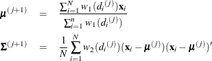
where ![]() is the M-distance evaluated at
is the M-distance evaluated at ![]() and
and ![]() obtained in the jth iteration. Carry out the iterations until
obtained in the jth iteration. Carry out the iterations until ![]() and
and ![]() converge. The final iteration yields the robust estimates of mean and covariance matrices. PROC CALIS uses the relative parameter
convergence criterion for the IRLS algorithm. The default criterion is 1E–8. See the XCONV=
option for the definition of the relative parameter convergence criterion. After the IRLS algorithm converges in the first
stage, the two-stage robust method proceeds to treat the robust mean and covariance estimates as if they were sample mean
and covariance matrices for a maximum likelihood estimation (METHOD=ML) of the model.
converge. The final iteration yields the robust estimates of mean and covariance matrices. PROC CALIS uses the relative parameter
convergence criterion for the IRLS algorithm. The default criterion is 1E–8. See the XCONV=
option for the definition of the relative parameter convergence criterion. After the IRLS algorithm converges in the first
stage, the two-stage robust method proceeds to treat the robust mean and covariance estimates as if they were sample mean
and covariance matrices for a maximum likelihood estimation (METHOD=ML) of the model.
The direct robust method computes the following residual M-distance ![]() for an observation with residual random vector
for an observation with residual random vector ![]() (say, of dimension
(say, of dimension ![]() , where h is the number of dependent observed variables
, where h is the number of dependent observed variables ![]() ):
):
where ![]() (
(![]() ) is a loading matrix that reduces
) is a loading matrix that reduces ![]() to
to ![]() independent components and q is the number of independent factors to be estimated from the dependent observed variables
independent components and q is the number of independent factors to be estimated from the dependent observed variables ![]() . The reduction of the residual vector into independent components is necessary when the number of factors q is not zero in the model. For
. The reduction of the residual vector into independent components is necessary when the number of factors q is not zero in the model. For ![]() , the residual covariance matrix
, the residual covariance matrix ![]() is not invertible and cannot be used in computing the residual M-distances. Hence, the covariance matrix
is not invertible and cannot be used in computing the residual M-distances. Hence, the covariance matrix ![]() of independent components
of independent components ![]() is used instead. See Yuan and Hayashi (2010) for details about the computation of the residuals in the context of structural equation modeling.
is used instead. See Yuan and Hayashi (2010) for details about the computation of the residuals in the context of structural equation modeling.
The direct robust method also computes two sets of weights as functions of the residual M-distances. Let ![]() be the M-distance of observation i, computed from the
be the M-distance of observation i, computed from the ![]() formula. The first set of weights
formula. The first set of weights ![]() applies to parameters in the first moments and is defined as
applies to parameters in the first moments and is defined as
The second set of weights ![]() applies to the parameters in the second moments and is defined as
applies to the parameters in the second moments and is defined as
These are essentially the same Huber-type weighting functions as those for the two-stage robust method. The only difference
is that the ![]() , instead of the
, instead of the ![]() , formula is used in the weighting functions for the direct robust method. The definition of
, formula is used in the weighting functions for the direct robust method. The definition of ![]() is also the same as that in the two-stage robust method, but it is now based on a different theoretical chi-square distribution.
That is, in the direct robust method,
is also the same as that in the two-stage robust method, but it is now based on a different theoretical chi-square distribution.
That is, in the direct robust method, ![]() is the critical value that corresponds to the
is the critical value that corresponds to the ![]() quantile of the
quantile of the ![]() distribution, with
distribution, with ![]() being the degrees of freedom. Again,
being the degrees of freedom. Again, ![]() is a tuning parameter and is set to 0.05 by default. You can override this value by using the ROBPHI=
option. The calculation of the number of "independent factors" q depends on the variants of the direct robust estimation that you choose. With the ROBUST=RES(E) option, q is the same as the number of exogenous factors specified in the model. With the ROBUST=RES(F) option, the disturbances of
the endogenous factors in the model are also treated as "independent factors," so q is the total number of latent factors specified in the model.
is a tuning parameter and is set to 0.05 by default. You can override this value by using the ROBPHI=
option. The calculation of the number of "independent factors" q depends on the variants of the direct robust estimation that you choose. With the ROBUST=RES(E) option, q is the same as the number of exogenous factors specified in the model. With the ROBUST=RES(F) option, the disturbances of
the endogenous factors in the model are also treated as "independent factors," so q is the total number of latent factors specified in the model.
The direct robust method (ROBUST=RES(E) or ROBUST=RES(F)) employs the IRLS algorithm in model estimation. Let the following
expression be a vector of nonredundant first and second moments structured in terms of model parameters ![]() :
:
where vech() extracts the lower-triangular nonredundant elements in ![]() . The updating formulas for
. The updating formulas for ![]() at the j+1 iteration is
at the j+1 iteration is
where ![]() is the parameter values at the jth iteration and
is the parameter values at the jth iteration and ![]() is defined by the following formula:
is defined by the following formula:
where ![]() is the model Jacobian,
is the model Jacobian, ![]() is the (normal theory) weight matrix for the moments (see Yuan and Zhong 2008 for the formula of the weight matrix), and
is the (normal theory) weight matrix for the moments (see Yuan and Zhong 2008 for the formula of the weight matrix), and ![]() is defined as
is defined as
Starting with some reasonable initial estimates for ![]() , PROC CALIS iterates the updating formulas until the relative parameter convergence criterion of the IRLS algorithm is satisfied.
The default criterion value is 1E–8. This essentially means that the IRLS algorithm converges when
, PROC CALIS iterates the updating formulas until the relative parameter convergence criterion of the IRLS algorithm is satisfied.
The default criterion value is 1E–8. This essentially means that the IRLS algorithm converges when ![]() is sufficiently small. See the XCONV=
option for the definition of the relative parameter convergence criterion.
is sufficiently small. See the XCONV=
option for the definition of the relative parameter convergence criterion.
Although the iterative formulas and the IRLS steps for robust estimation have been presented for single-group analysis, they
are easily generalizable to multiple-group analysis. For the two-stage robust method, you only need to repeat the robust estimation
of the means and covariances for the groups and then apply the obtained robust moments as if they were sample moments for
regular maximum likelihood estimation (METHOD=ML). For the direct robust method, you need to expand the dimensions of the
model Jacobian matrix ![]() , the weight matrix
, the weight matrix ![]() , and the vector
, and the vector ![]() to include moments from several groups/models. Therefore, the multiple-group formulas are conceptually quite simple but tedious
to present. For this reason, they are omitted here.
to include moments from several groups/models. Therefore, the multiple-group formulas are conceptually quite simple but tedious
to present. For this reason, they are omitted here.