The CALIS Procedure
-
Overview

-
Getting Started
-
SyntaxClasses of Statements in PROC CALISSingle-Group Analysis SyntaxMultiple-Group Multiple-Model Analysis SyntaxPROC CALIS StatementBOUNDS StatementBY StatementCOSAN StatementCOV StatementDETERM StatementEFFPART StatementFACTOR StatementFITINDEX StatementFREQ StatementGROUP StatementLINCON StatementLINEQS StatementLISMOD StatementLMTESTS StatementMATRIX StatementMEAN StatementMODEL StatementMSTRUCT StatementNLINCON StatementNLOPTIONS StatementOUTFILES StatementPARAMETERS StatementPARTIAL StatementPATH StatementPATHDIAGRAM StatementPCOV StatementPVAR StatementRAM StatementREFMODEL StatementRENAMEPARM StatementSAS Programming StatementsSIMTESTS StatementSTD StatementSTRUCTEQ StatementTESTFUNC StatementVAR StatementVARIANCE StatementVARNAMES StatementWEIGHT Statement
-
DetailsInput Data SetsOutput Data SetsDefault Analysis Type and Default ParameterizationThe COSAN ModelThe FACTOR ModelThe LINEQS ModelThe LISMOD Model and SubmodelsThe MSTRUCT ModelThe PATH ModelThe RAM ModelNaming Variables and ParametersSetting Constraints on ParametersAutomatic Variable SelectionPath Diagrams: Layout Algorithms, Default Settings, and CustomizationEstimation CriteriaRelationships among Estimation CriteriaGradient, Hessian, Information Matrix, and Approximate Standard ErrorsCounting the Degrees of FreedomAssessment of FitCase-Level Residuals, Outliers, Leverage Observations, and Residual DiagnosticsTotal, Direct, and Indirect EffectsStandardized SolutionsModification IndicesMissing Values and the Analysis of Missing PatternsMeasures of Multivariate KurtosisInitial EstimatesUse of Optimization TechniquesComputational ProblemsDisplayed OutputODS Table NamesODS Graphics
-
ExamplesEstimating Covariances and CorrelationsEstimating Covariances and Means SimultaneouslyTesting Uncorrelatedness of VariablesTesting Covariance PatternsTesting Some Standard Covariance Pattern HypothesesLinear Regression ModelMultivariate Regression ModelsMeasurement Error ModelsTesting Specific Measurement Error ModelsMeasurement Error Models with Multiple PredictorsMeasurement Error Models Specified As Linear EquationsConfirmatory Factor ModelsConfirmatory Factor Models: Some VariationsResidual Diagnostics and Robust EstimationThe Full Information Maximum Likelihood MethodComparing the ML and FIML EstimationPath Analysis: Stability of AlienationSimultaneous Equations with Mean Structures and Reciprocal PathsFitting Direct Covariance StructuresConfirmatory Factor Analysis: Cognitive AbilitiesTesting Equality of Two Covariance Matrices Using a Multiple-Group AnalysisTesting Equality of Covariance and Mean Matrices between Independent GroupsIllustrating Various General Modeling LanguagesTesting Competing Path Models for the Career Aspiration DataFitting a Latent Growth Curve ModelHigher-Order and Hierarchical Factor ModelsLinear Relations among Factor LoadingsMultiple-Group Model for Purchasing BehaviorFitting the RAM and EQS Models by the COSAN Modeling LanguageSecond-Order Confirmatory Factor AnalysisLinear Relations among Factor Loadings: COSAN Model SpecificationOrdinal Relations among Factor LoadingsLongitudinal Factor Analysis
- References
There is always some arbitrariness to classify the estimation methods according to certain mathematical or numerical properties. The discussion in this section is not meant to be a thorough classification of the estimation methods available in PROC CALIS. Rather, classification is done here with the purpose of clarifying the uses of different estimation methods and the theoretical relationships of estimation criteria.
GLS, ML, and FIML assume multivariate normality of the data, while ULS, WLS, and DWLS do not. Although the ML method with covariance structure analysis alone can also be based on the Wishart distribution of the sample covariance matrix, for convenience GLS, ML, and FIML are usually classified as normal-theory based methods, while ULS, WLS, and DWLS are usually classified as distribution-free methods.
An intuitive or even naive notion is usually that methods without distributional assumptions such as WLS and DWLS are preferred to normal theory methods such as ML and GLS in practical situations where multivariate normality is doubt. This notion might need some qualifications because there are simply more factors to consider in judging the quality of estimation methods in practice. For example, the WLS method might need a very large sample size to enjoy its purported asymptotic properties, while the ML might be robust against the violation of multi-normality assumption under certain circumstances. No recommendations regarding which estimation criterion should be used are attempted here, but you should make your choice based more than the assumption of multivariate normality.
If only the covariance or correlation structures are considered, the six estimation functions, ![]() ,
, ![]() ,
, ![]() ,
, ![]() ,
, ![]() , and
, and ![]() , belong to the following two groups:
, belong to the following two groups:
-
The functions
 ,
,  ,
,  , and
, and  take into account all
  elements of the symmetric residual matrix
  . This means that the off-diagonal residuals contribute twice to the discrepancy function F, as lower and as upper triangle elements.
-
The functions
 and
and  take into account only the
  lower triangular elements of the symmetric residual matrix . This means that the off-diagonal residuals contribute to the discrepancy function F only once.
The ![]() function used in PROC CALIS differs from that used by the LISREL 7 program. Formula (1.25) of the LISREL 7 manual (Jöreskog
and Sörbom, 1985, p. 23) shows that LISREL groups the
function used in PROC CALIS differs from that used by the LISREL 7 program. Formula (1.25) of the LISREL 7 manual (Jöreskog
and Sörbom, 1985, p. 23) shows that LISREL groups the ![]() function in the first group by taking into account all
function in the first group by taking into account all ![]() elements of the symmetric residual matrix
elements of the symmetric residual matrix ![]() .
.
-
Relationship between DWLS and WLS: PROC CALIS: The
and discrepancy functions deliver the same results for the special case that the weight matrix  used by WLS estimation is a diagonal matrix. LISREL 7: This is not the case.
-
Relationship between DWLS and ULS: LISREL 7: The
and estimation functions deliver the same results for the special case that the diagonal weight matrix used by DWLS estimation is an identity matrix. PROC CALIS: To obtain the same results with and estimation, set the diagonal weight matrix used in DWLS estimation to:
![\[ [\mb{W}_{ss}]_{ik,ik} = \left\{ \begin{array}{llll} 1. & \mbox{if $i = k$} & & \\ 0.5 & \mbox{otherwise} & & \mbox{($k \le i$)} \end{array} \right. \]](images/statug_calis0585.png)
Because the reciprocal elements of the weight matrix are used in the discrepancy function, the off-diagonal residuals are weighted by a factor of 2.
Both the ML and FIML methods can be derived from the log-likelihood function for multivariate normal data. The preceding
section Estimation Criteria mentions that ![]() is essentially the same as
is essentially the same as ![]() , where L is the log-likelihood function for multivariate normal data. For the ML estimation, you can also consider
, where L is the log-likelihood function for multivariate normal data. For the ML estimation, you can also consider ![]() as a part of the
as a part of the ![]() discrepancy function that contains the information regarding the model parameters (while the rest the
discrepancy function that contains the information regarding the model parameters (while the rest the ![]() function contains some constant terms given the data). That is, with some algebraic manipulations and assuming that there
is no missing value in the analysis (so that all
function contains some constant terms given the data). That is, with some algebraic manipulations and assuming that there
is no missing value in the analysis (so that all ![]() and
and ![]() are the same as
are the same as ![]() and
and ![]() , respectively), it can shown that
, respectively), it can shown that
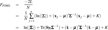
where ![]() is the sample mean and
is the sample mean and ![]() is the biased sample covariance matrix. Compare this FIML function with the ML function shown in the following expression,
which shows that both functions are very similar:
is the biased sample covariance matrix. Compare this FIML function with the ML function shown in the following expression,
which shows that both functions are very similar:
The two expressions differ only in the constant terms, which are independent of the model parameters, and in the formulas for computing the sample covariance matrix. While the FIML method assumes the biased formula (with N as the divisor, by default) for the sample covariance matrix, the ML method (as implemented in PROC CALIS) uses the unbiased formula (with N – 1 as the divisor, by default).
The similarity (or dissimilarity) of the ML and FIML discrepancy functions leads to some useful conclusions here:
-
Because the constant terms in the discrepancy functions play no part in parameter estimation (except for shifting the function values), overriding the default ML method with VARDEF =N (that is, using N as the divisor in the covariance matrix formula) leads to the same estimation results as that of the FIML method, given that there are no missing values in the analysis.
-
Because the FIML function is evaluated at the level of individual observations, it is much more expensive to compute than the ML function. As compared with ML estimation, FIML estimation takes longer and uses more computing resources. Hence, for data without missing values, the ML method should always be chosen over the FIML method.
-
The advantage of the FIML method lies solely in its ability to handle data with random missing values. While the FIML method uses the information maximally from each observation, the ML method (as implemented in PROC CALIS) simply throws away any observations with at least one missing value. If it is important to use the information from observations with random missing values, the FIML method should be given consideration over the ML method.
See Example 29.15 for an application of the FIML method and Example 29.16 for an empirical comparison of the ML and FIML methods. For more examples and details about the FIML method employed by PROC CALIS, see Yung and Zhang (2011); Zhang and Yung (2011).