The CALIS Procedure
-
Overview

-
Getting Started
-
SyntaxClasses of Statements in PROC CALISSingle-Group Analysis SyntaxMultiple-Group Multiple-Model Analysis SyntaxPROC CALIS StatementBOUNDS StatementBY StatementCOSAN StatementCOV StatementDETERM StatementEFFPART StatementFACTOR StatementFITINDEX StatementFREQ StatementGROUP StatementLINCON StatementLINEQS StatementLISMOD StatementLMTESTS StatementMATRIX StatementMEAN StatementMODEL StatementMSTRUCT StatementNLINCON StatementNLOPTIONS StatementOUTFILES StatementPARAMETERS StatementPARTIAL StatementPATH StatementPATHDIAGRAM StatementPCOV StatementPVAR StatementRAM StatementREFMODEL StatementRENAMEPARM StatementSAS Programming StatementsSIMTESTS StatementSTD StatementSTRUCTEQ StatementTESTFUNC StatementVAR StatementVARIANCE StatementVARNAMES StatementWEIGHT Statement
-
DetailsInput Data SetsOutput Data SetsDefault Analysis Type and Default ParameterizationThe COSAN ModelThe FACTOR ModelThe LINEQS ModelThe LISMOD Model and SubmodelsThe MSTRUCT ModelThe PATH ModelThe RAM ModelNaming Variables and ParametersSetting Constraints on ParametersAutomatic Variable SelectionPath Diagrams: Layout Algorithms, Default Settings, and CustomizationEstimation CriteriaRelationships among Estimation CriteriaGradient, Hessian, Information Matrix, and Approximate Standard ErrorsCounting the Degrees of FreedomAssessment of FitCase-Level Residuals, Outliers, Leverage Observations, and Residual DiagnosticsTotal, Direct, and Indirect EffectsStandardized SolutionsModification IndicesMissing Values and the Analysis of Missing PatternsMeasures of Multivariate KurtosisInitial EstimatesUse of Optimization TechniquesComputational ProblemsDisplayed OutputODS Table NamesODS Graphics
-
ExamplesEstimating Covariances and CorrelationsEstimating Covariances and Means SimultaneouslyTesting Uncorrelatedness of VariablesTesting Covariance PatternsTesting Some Standard Covariance Pattern HypothesesLinear Regression ModelMultivariate Regression ModelsMeasurement Error ModelsTesting Specific Measurement Error ModelsMeasurement Error Models with Multiple PredictorsMeasurement Error Models Specified As Linear EquationsConfirmatory Factor ModelsConfirmatory Factor Models: Some VariationsResidual Diagnostics and Robust EstimationThe Full Information Maximum Likelihood MethodComparing the ML and FIML EstimationPath Analysis: Stability of AlienationSimultaneous Equations with Mean Structures and Reciprocal PathsFitting Direct Covariance StructuresConfirmatory Factor Analysis: Cognitive AbilitiesTesting Equality of Two Covariance Matrices Using a Multiple-Group AnalysisTesting Equality of Covariance and Mean Matrices between Independent GroupsIllustrating Various General Modeling LanguagesTesting Competing Path Models for the Career Aspiration DataFitting a Latent Growth Curve ModelHigher-Order and Hierarchical Factor ModelsLinear Relations among Factor LoadingsMultiple-Group Model for Purchasing BehaviorFitting the RAM and EQS Models by the COSAN Modeling LanguageSecond-Order Confirmatory Factor AnalysisLinear Relations among Factor Loadings: COSAN Model SpecificationOrdinal Relations among Factor LoadingsLongitudinal Factor Analysis
- References
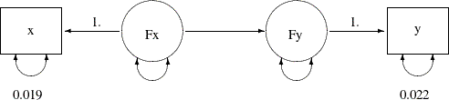
In Example 29.8, you fit a simple measurement error model with errors in both of the predictor variable x and the outcome variable y. From prior studies, the measurement error variance of x is 0.019 and the measurement error variance of y is 0.022. You use the following path diagram to represent the model:
With this path diagram, you use the PATH modeling language of PROC CALIS to specify the model, as shown in the following:
proc calis data=measures;
   path
      x  <=== Fx  = 1.,
      Fx ===> Fy   ,
      Fy ===> y   = 1.;
   pvar
      x  = 0.019,
      y  = 0.022,
      Fx Fy;
run;
In the path diagram and in the PATH model specification, there are no explicit representations of the error terms in the model.
You express the error variances of x, y, and Fy as partial variances of the endogenous variables. In the path diagram, you represent these partial variances by the double-headed
arrows. Correspondingly, in the PATH statement of PROC CALIS, you specify these partial variances in the PVAR statement.
In practice, some researchers might prefer to express the error terms in the model explicitly. For example, with the error terms added to the preceding measurement error model, the new path diagram becomes:
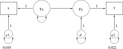
In the path diagram, you add paths from error variables e1, e2, and d to the endogenous variables x, y, and Fy, respectively. All these paths from the error terms have a fixed path coefficient of 1. The error variances are represented
by double-headed arrows directly attached to them. For example, the variance of e1 is fixed at 0.019, and the variance of e2 is fixed at 0.022. The variance of d, which is sometime called the disturbance, is a free unnamed parameter in the path diagram. Similarly, the variance of Fx is a free unnamed parameter in the model.
Corresponding to this new path diagram, you can use the LINEQS modeling language for specifying your model in PROC CALIS, as shown in the following statements:
proc calis data=measures;
   lineqs
      x   = 1. * Fx  +  e1,
      y   = 1. * Fy  +  e2,
      Fy  =    * Fx  +   d;
   variance
      e1  = 0.019,
      e2  = 0.022,
      Fx d;
run;
The LINEQS model specification in PROC CALIS emphasizes the linear equation input. In each of the linear equations in the
LINEQS statement, you specify an endogenous variable and how it is related to other variables. An endogenous variable in the
path diagram is a variable that has at least one single-headed arrow pointing to it. You need to list all endogenous variables
on the left-hand side of the linear equations of the LINEQS statement. In the current model, variables x, y, and Fy are endogenous, and therefore you specify three linear equations in the LINEQS statement. The first two equations represent
the measurement model for the observed variables, while the third equation represents the structural equation of the model.
Notice that in the third equation, you do not specify the path coefficient that is attached to Fx. PROC CALIS treats unspecified path coefficients as free parameters. The effect of Fx on Fy is freely estimated, as required in the path diagram representation.
In the VARIANCE statement, you specify the variances of the exogenous variables in the model. The specifications in the VARIANCE
statement of the LINEQS model are very similar to those in the PVAR statement of the PATH model. The main difference is the
use of error variable names in the VARIANCE statement. With the LINEQS model specification, you can only specify exogenous
variables in the VARIANCE statement. Hence, you must specify the error variables e1, e2, and d in the VARIANCE statement of the LINEQS model, instead of the corresponding endogenous variables x, y, and Fy in the PVAR statement of the PATH model.
Output 29.11.3 shows the parameter estimates of the LINEQS model.
All these estimates are essentially the same as those obtained from the PATH model specification, as shown in Output 29.11.4.
You can use either the LINEQS or PATH model specification in PROC CALIS for your analysis problems. They give you the same estimation results.
So far the measurement error model is concerned with one predictor. With more predictors in the model, you might also want
to model the correlated measurement errors in the x variables. You can analyze this kind of model by using the PATH model specification, as shown in Example 29.10. With measurement error terms explicitly assumed, you can also use the LINEQS model specification. This example illustrates
how you can do that by using the same data set and the measurement error model with correlated errors in Example 29.10.
In the data set, you have four observed variables: x1–x3 and y. All are measured with errors, as represented by the following path diagram:
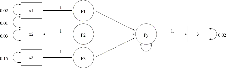
In the path diagram, F1–F3 and Fy represent true scores for the measurement indicators x1–x3 and y, respectively. You predict Fy by F1–F3, which represents the structural relationships in the model. Measurement error variances of the observed variables are treated
as known and are represented by the double-headed arrows attached to the observed variables. For example, the error variance
of x3 is 0.15. In addition, the error covariance between x1 and x2 is treated as known. The double-headed arrow that connects x1 and x2 represents the error covariance, and this covariance is fixed at 0.01 in the model.
You transcribe this path diagram representation into the following PATH model specification:
proc calis data=multiple nobs=37;
   path
      Fy  <===   F1 F2 F3,
      F1  ===>   x1   = 1.,
      F2  ===>   x2   = 1.,
      F3  ===>   x3   = 1.,
      Fy  ===>   y    = 1.;
   pvar
      x1 x2 x3 y = .02 .03 .15 .02,
      Fy;
   pcov
      x1 x2 = 0.01;
run;
To represent the error terms explicitly, you can add the error terms to the path diagram with some modifications, as shown in the following:
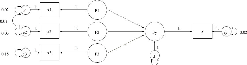
In the path diagram, you attach error variables e1–e3, ey, and d to the associated endogenous variables in the model. The error variances and covariances, which are attached to the endogenous
variables directly, are now attached to the corresponding error variables. With this new path diagram, you can use the following
LINEQS model specification for the model:
proc calis data=multiple nobs=37;
   lineqs
      Fy =     * F1 +  * F2 +  * F3 + d,
      x1 =  1. * F1 + e1,
      x2 =  1. * F2 + e2,
      x3 =  1. * F3 + e3,
       y =  1. * Fy + ey;
    variance
       e1-e3 ey = .02 .03 .15 .02,
       d;
    cov
       e1 e2 = 0.01;
run;
Again, in each linear equation of the LINEQS statement, you specify the functional relationship of an endogenous variable
with other variables, including the error variable. The first equation is the structural equation in the model. You want to
estimate the effects of F1, F2, and F3 on Fy. The error or disturbance variable is d. In the next four equations, you relate the observed variables with their true scores counterparts.
In the VARIANCE statement, you specify the error variances with reference to the error variables in the path diagram. Four
of the error variances are fixed constants, as required in the model. The last specification represents a free parameter for
the variance of d. The specifications in the VARIANCE statement of the LINEQS model are similar to those in the PVAR statement of the PATH
model specification. The difference is that in the PATH model specification the reference variables are the endogenous variables
in the PATH model, while in the LINEQS model specification the reference variables are the associated error variables.
In the COV statement, you specify the covariance between the error variables e1 and e2. Again, this is similar to the corresponding specification of the PATH model, where the same error covariance is specified
as the partial covariance between x1 and x2 in the PCOV statement.
Output 29.11.7 shows the parameter estimates that result from using the LINEQS model specification. Estimates in the equations, variances, and covariances are shown respectively.
Output 29.11.7: Parameter Estimates of the Measurement Model with Multiple Predictors: LINEQS Model
| Estimates for Variances of Exogenous Variables | ||||||
|---|---|---|---|---|---|---|
| Variable Type |
Variable | Parameter | Estimate | Standard Error |
t Value | Pr > |t| |
| Error | e1 | 0.02000 | ||||
| e2 | 0.03000 | |||||
| e3 | 0.15000 | |||||
| ey | 0.02000 | |||||
| Disturbance | d | _Parm4 | 0.16421 | 0.04523 | 3.6305 | 0.0003 |
| Latent | F1 | _Add1 | 1.40000 | 0.33470 | 4.1829 | <.0001 |
| F2 | _Add2 | 1.12000 | 0.27106 | 4.1320 | <.0001 | |
| F3 | _Add3 | 13.96000 | 3.32576 | 4.1975 | <.0001 | |
Output 29.11.8 shows the parameter estimates that result from using the PATH model specification. The estimates in the path list shown in Output 29.11.8 correspond to those of the equation output in Output 29.11.7. The variance estimates in Output 29.11.8 correspond to those variance estimates of the exogenous variables of the LINEQS model, as shown in Output 29.11.7. Finally, the last two tables in Output 29.11.8 correspond to the covariance estimates among the exogenous variables of the LINEQS model, as shown in Output 29.11.7. Again, the LINEQS and PATH model specification give you exactly the same estimation results, but in different output formats.
Output 29.11.8: Parameter Estimates of the Measurement Model with Multiple Predictors: PATH Model
| Variance Parameters | ||||||
|---|---|---|---|---|---|---|
| Variance Type |
Variable | Parameter | Estimate | Standard Error |
t Value | Pr > |t| |
| Error | x1 | 0.02000 | ||||
| x2 | 0.03000 | |||||
| x3 | 0.15000 | |||||
| y | 0.02000 | |||||
| Fy | _Parm4 | 0.16421 | 0.04523 | 3.6305 | 0.0003 | |
| Exogenous | F1 | _Add1 | 1.40000 | 0.33470 | 4.1829 | <.0001 |
| F2 | _Add2 | 1.12000 | 0.27106 | 4.1320 | <.0001 | |
| F3 | _Add3 | 13.96000 | 3.32576 | 4.1975 | <.0001 | |
In this example, you fit measurement error models by using the LINEQS and PATH model specifications of PROC CALIS. The two different model specification languages give you essentially the same estimation results. The measurement models can have multiple true scores predictors and correlated errors. The measurement error models considered so far have only one measured indicator for each true score latent variable. This is usually not the case in many psychometric or sociological applications where latent factors usually have several observed indicators. The confirmatory factor model is a typical example of this kind of applications. See Example 29.12 for an application of PROC CALIS to fit confirmatory factor models. See Example 29.17 for an application of PROC CALIS to fit a general structural equation model where latent variables have more than one measured indicators.