Example 29.13 Confirmatory Factor Models: Some Variations
This example shows how you can fit some variations of the basic confirmatory factor analysis model by the FACTOR modeling
language. You apply these models to the scores data set that is described in Example 29.12. The data set contains six test scores of verbal and math abilities. Thirty-two students take the tests. Tests x1–x3 test their verbal skills and tests y1–y3 test their math skills.
In classical measurement theory, test items for a latent factor are parallel if they have the same loadings on the factor
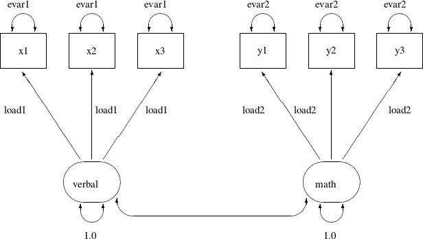
and the same error variances (or reliability). Suppose for the scores data, the items within each of the verbal and the math factors are parallel. You can use the following path diagram to represent such a parallel tests model:
In the path diagram, the variances of the verbal and the math are both fixed at 1, as indicated by the constants 1.0 adjacent to the double-headed arrows that are attached to factors.
You label all the single-headed paths in the path diagram by parameter names. For the three paths (loadings) from the verbal factor, you use the same parameter name load1. This means that these loadings are the same parameter. You also label the double-headed arrows that are attached to x1–x3 by the parameter name evar1. This means that the corresponding error variances for these three observed variables are exactly the same. Hence, x1–x3 are parallel tests for the verbal factor, as required by the current confirmatory factor model.
Similarly, you define parallel tests y1–y3 for the math factor by using load2 as the common factor loading parameter and evar2 as the common error variances for the observed variables.
Corresponding to this path diagram, you can specify the model by the following FACTOR model specification of PROC CALIS:
proc calis data=scores;
   factor
      verbal ===> x1-x3   = load1 load1 load1,
      math   ===> y1-y3   = load2 load2 load2;
   pvar
      verbal = 1.,
      math   = 1.,
      x1-x3  = 3*evar1,
      y1-y3  = 3*evar2;
run;
In each entry of the FACTOR statement, you specify the factor-variables relationships, followed by a list of parameters. For
example, the three loading parameters of x1–x3 on the verbal factor are all named load1. This effectively constrains the corresponding loading estimates to be the same. Similarly, in the next entry you set equality
constraints on the loading estimates y1–y3 on the math factor by using the same parameter name load2.
To make the tests parallel, you also need to constrain the error variances for each variable cluster. In the PVAR statement,
in addition to setting the factor variances to 1 for identification, you set all the error variances of x1–x3 to be the same by using the same parameter name evar1. The notation 3*evar1 means that you want to specify evar1 three times, one time each for the error variances for the three observed variables in the variable list of the entry. Similarly,
you set the equality of the error variances of y1–y3 by using the same parameter name evar2.
Output 29.13.2 shows some fit indices of the parallel tests model for the scores data. The model fit chi-square is 26.128 (df = 16, p = 0.0522). The SRMR value is 0.1537 and the RMSEA value is 0.1429. All these indices show that the model does not fit very
well. However, Bentler’s CFI is 0.9366, which shows a good model fit.
Output 29.13.2: Model Fit of the Parallel Tests Model: Scores Data
| 26.1283 |
| 16 |
| 0.0522 |
| 0.1537 |
| 0.1429 |
| 0.9366 |
Output 29.13.3 shows the parameter estimates of the parallel tests model. The first table of Output 29.13.3 shows the required factor pattern for parallel tests. Variables x1–x3 all have the same loading estimates on the verbal factor, and variables y1–y3 all have the same loading estimates on the math factor. All loading estimates are statistically significant.
Output 29.13.3: Parameter Estimates of the Parallel Tests Model: Scores Data
| 5.4226 |
| 0.7655 |
| 7.0833 |
| <.0001 |
| [load1] |
|
|
| 5.4226 |
| 0.7655 |
| 7.0833 |
| <.0001 |
| [load1] |
|
|
| 5.4226 |
| 0.7655 |
| 7.0833 |
| <.0001 |
| [load1] |
|
|
|
|
| 4.4001 |
| 0.5926 |
| 7.4246 |
| <.0001 |
| [load2] |
|
|
|
| 4.4001 |
| 0.5926 |
| 7.4246 |
| <.0001 |
| [load2] |
|
|
|
| 4.4001 |
| 0.5926 |
| 7.4246 |
| <.0001 |
| [load2] |
|
|
|
| 0.5024 |
| 0.1497 |
| 3.3569 |
| 0.000788 |
| [_Add1] |
|
| 0.5024 |
| 0.1497 |
| 3.3569 |
| 0.000788 |
| [_Add1] |
|
|
| evar1 |
9.61122 |
1.72623 |
5.5678 |
<.0001 |
| evar1 |
9.61122 |
1.72623 |
5.5678 |
<.0001 |
| evar1 |
9.61122 |
1.72623 |
5.5678 |
<.0001 |
| evar2 |
3.46673 |
0.62264 |
5.5678 |
<.0001 |
| evar2 |
3.46673 |
0.62264 |
5.5678 |
<.0001 |
| evar2 |
3.46673 |
0.62264 |
5.5678 |
<.0001 |
In the second table of Output 29.13.3, the factor covariance (or correlation) estimate is 0.5024, showing moderate relationship between the verbal and the math factors. The last table of Output 29.13.3 shows the error variances of the variables. As required by the parallel tests model, the error variance estimates of x1–x3 are all 9.6112, and the error variance estimates of y1–y3 are all 3.4667.
The Tau-Equivalent Tests Model
Because the parallel tests model does not fit well, you are looking for a less constrained model for the scores data. The tau-equivalent tests model is such a model. It requires only the equality of factor loadings but not the equality
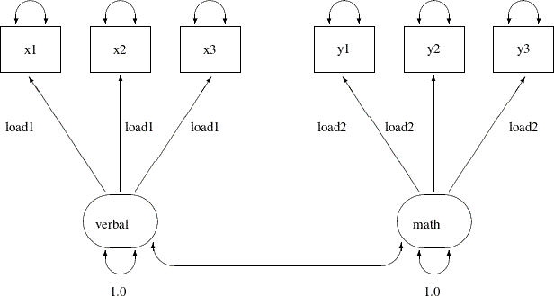
of error variances within each factor. The following path diagram represents the tau-equivalent tests model for the scores data:
This path diagram is much the same as that for the parallel tests model except that now you do not use parameter names to
label the double-headed arrows that are attached to the observed variables. This means that you allow the corresponding error
variances to be free parameters in the tau-equivalent tests model. You can use the following FACTOR model specification of
PROC CALIS to specify the tau-equivalent tests model for the scores data:
proc calis data=scores;
   factor
      verbal ===> x1-x3   = load1 load1 load1,
      math   ===> y1-y3   = load2 load2 load2;
   pvar
      verbal = 1.,
      math   = 1.;
run;
This specification is the same as that for the parallel tests model except that you remove the specifications about the error
variances in the PVAR statement in the current tau-equivalent model. This effectively allows the error variances of the observed
variables to be (default) free parameters in the model.
Output 29.13.5 shows some model fit indices of the tau-equivalent tests model for the scores data. The chi-square is 22.0468 (df = 12, p = 0.037). The SRMR is 0.1398 and the RMSEA is 0.1643. The comparative fit index (CFI) is 0.9371. Except for the CFI value,
all other values do not support a good model fit. This model has a degrees of freedom of 12, which is less restrictive (has
more parameters) than the parallel tests model, which has a degrees of freedom of 16, as shown in Output 29.13.2. However, it seems that the tau-equivalent tests model is still too restrictive for the data.
Output 29.13.5: Model Fit of the Tau-Equivalent Tests Model: Scores Data
| 22.0468 |
| 12 |
| 0.0370 |
| 0.1398 |
| 0.1643 |
| 0.9371 |
Output 29.13.6 shows the parameter estimates. The first table of Output 29.13.6 shows the required pattern of factor loadings under the tau-equivalent tests model. The third table of Output 29.13.6 shows the error variance estimates. The error variance parameters are no longer constrained under the tau-equivalent tests
model. Each has a unique estimate.
Output 29.13.6: Parameter Estimates of the Tau-Equivalent Tests Model: Scores Data
| 5.2418 |
| 0.7374 |
| 7.1085 |
| <.0001 |
| [load1] |
|
|
| 5.2418 |
| 0.7374 |
| 7.1085 |
| <.0001 |
| [load1] |
|
|
| 5.2418 |
| 0.7374 |
| 7.1085 |
| <.0001 |
| [load1] |
|
|
|
|
| 4.4462 |
| 0.5932 |
| 7.4953 |
| <.0001 |
| [load2] |
|
|
|
| 4.4462 |
| 0.5932 |
| 7.4953 |
| <.0001 |
| [load2] |
|
|
|
| 4.4462 |
| 0.5932 |
| 7.4953 |
| <.0001 |
| [load2] |
|
|
|
| 0.4514 |
| 0.1569 |
| 2.8772 |
| 0.004012 |
| [_Add1] |
|
| 0.4514 |
| 0.1569 |
| 2.8772 |
| 0.004012 |
| [_Add1] |
|
|
| _Add2 |
13.05681 |
4.19549 |
3.1121 |
0.0019 |
| _Add3 |
10.80421 |
3.70322 |
2.9175 |
0.0035 |
| _Add4 |
5.43527 |
2.72147 |
1.9972 |
0.0458 |
| _Add5 |
3.29858 |
1.24673 |
2.6458 |
0.0082 |
| _Add6 |
1.90435 |
1.02393 |
1.8598 |
0.0629 |
| _Add7 |
5.09724 |
1.61477 |
3.1566 |
0.0016 |
The Partially Constrained Parallel Tests Model
Because both the parallel tests and tau-equivalent tests models do not fit the data well, you can explore an alternative
model for the scores data. Suppose that for each factor only two (but not all) of their measured variables (tests) are parallel. For example,
suppose you know that tests x1 and x2 are very similar to each other (for example, both are speeded tests with forced-choice answers), while x3 is a little different in the way it is administered (for example, open-ended questions). Although all tests are designed
for measuring the verbal factor, only x1 and x2 are parallel tests while x3 is congeneric to the verbal factor. Similarly, suppose you can argue that y2 and y3 are parallel tests while y1 is only congeneric to the math factor.
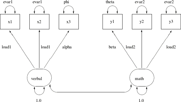
The current modeling idea is represented by the following path diagram:
In the path diagram, x1 and x2 have the same parameter load1 for the paths from the verbal factor. Their error variances are also the same, as labeled with the evar1 parameter adjacent to the double-headed arrows that are attached to the variables. The test x3 has distinct parameter names for its associated path and the attached double-headed arrow. The corresponding loading and
error variance parameters are alpha and phi, respectively. Similarly, with the use of specific parameter names, you define y2 and y3 as parallel tests for the math factor, while y1 is congeneric to the same factor but with distinct loading and error variance parameters. Lastly, you fix the variances of
the factors to 1.0 for identification of the factor scales.
You can specify such a partially constrained parallel tests model by the following FACTOR model specification of PROC CALIS:
proc calis data=scores;
   factor
      verbal ===> x1-x3   = load1 load1 alpha,
      math   ===> y1-y3   = beta  load2 load2;
   pvar
      verbal = 1.,
      math   = 1.,
      x1-x3  = evar1  evar1  phi,
      y1-y3  = theta  evar2  evar2;
run;
First, in the FACTOR statement, you name the loading parameters that reflect the parallel tests constraints. For example,
the loading parameters of x1 and x2 on the verbal factor are both named load1. This means that they are the same. However, the loading parameter of x3 on the verbal factor is named alpha, which means that it is a separate parameter. Similarly, you apply the load2 parameter name to the loading parameters of y2 and y3 on the math factor, but the loading parameter of y1 on the math factor is a distinct parameter named beta.
In the PVAR statement, the two factor variances are set to a constant 1 for the identification of latent factor scales. Next,
you use the same naming techniques as in the FACTOR statement to constrain some parts of the error variances. As a result,
together with the specifications in the FACTOR statement, x1 and x2 are parallel tests for the verbal factor and y2 and y3 are parallel tests for the math factor, while x3 and y1 are only congeneric tests for their respective factors.
Output 29.13.8 shows some fit indices of the partially constrained parallel tests model. The model fit chi-square is 12.6784 (df = 12, p = 0.3928). The SRMR is 0.0585 and the RMSEA is close to 0.0427. The comparative fit index (CFI) is 0.9958. All these fit
indices point to a quite reasonable model fit for the scores data.
Output 29.13.8: Model Fit of the Partially Constrained Parallel Tests Model: Scores Data
| 12.6784 |
| 12 |
| 0.3928 |
| 0.0585 |
| 0.0427 |
| 0.9958 |
Notice that the current model actually has the same degrees of freedom as that of the tau-equivalent tests model, as shown
in Output 29.13.5. Both models have nine parameters. But the current partially constrained parallel tests model is definitely a better model
for the data. This shows that sometimes you do not have to add more parameters to improve the model fit. Structurally different
models might explain the data quite differently, even though they might use the same number of parameters.
Output 29.13.9 show the parameter estimates of the partially constrained parallel tests model for the scores data. The estimates in the factor loading matrix and error variances table confirm the prescribed nature of the tests—that
is, x1 and x2 are parallel tests for the verbal factor and y2 and y3 are parallel tests for the math factor.
Output 29.13.9: Parameter Estimates of the Partially Constrained Parallel Tests Model: Scores Data
| 5.8306 |
| 0.8593 |
| 6.7853 |
| <.0001 |
| [load1] |
|
|
| 5.8306 |
| 0.8593 |
| 6.7853 |
| <.0001 |
| [load1] |
|
|
| 4.6623 |
| 0.7814 |
| 5.9664 |
| <.0001 |
| [alpha] |
|
|
|
|
| 5.2784 |
| 0.7010 |
| 7.5294 |
| <.0001 |
| [beta] |
|
|
|
| 3.9789 |
| 0.5732 |
| 6.9419 |
| <.0001 |
| [load2] |
|
|
|
| 3.9789 |
| 0.5732 |
| 6.9419 |
| <.0001 |
| [load2] |
|
|
|
| 0.5203 |
| 0.1425 |
| 3.6497 |
| 0.000263 |
| [_Add1] |
|
| 0.5203 |
| 0.1425 |
| 3.6497 |
| 0.000263 |
| [_Add1] |
|
|
| evar1 |
10.31998 |
2.57827 |
4.0027 |
<.0001 |
| evar1 |
10.31998 |
2.57827 |
4.0027 |
<.0001 |
| phi |
6.67832 |
2.59902 |
2.5696 |
0.0102 |
| theta |
0.80714 |
1.35247 |
0.5968 |
0.5506 |
| evar2 |
4.07534 |
1.00371 |
4.0603 |
<.0001 |
| evar2 |
4.07534 |
1.00371 |
4.0603 |
<.0001 |