The REG Procedure
- Overview
-
Getting Started

-
Syntax
-
DetailsMissing ValuesInput Data SetsOutput Data SetsInteractive AnalysisModel-Selection MethodsCriteria Used in Model-Selection MethodsLimitations in Model-Selection MethodsParameter Estimates and Associated StatisticsPredicted and Residual ValuesModels of Less Than Full RankCollinearity DiagnosticsModel Fit and Diagnostic StatisticsInfluence StatisticsReweighting Observations in an AnalysisTesting for HeteroscedasticityTesting for Lack of FitMultivariate TestsAutocorrelation in Time Series DataComputations for Ridge Regression and IPC AnalysisConstruction of Q-Q and P-P PlotsComputational MethodsComputer Resources in Regression AnalysisDisplayed OutputPlot Options Superseded by ODS GraphicsODS Table NamesODS Graphics
-
Examples
- References
Consider a response variable Y that can be predicted by a polynomial function of a regressor variable X. You can estimate ![]() , the intercept;
, the intercept; ![]() , the slope due to X; and
, the slope due to X; and ![]() , the slope due to
, the slope due to ![]() , in
, in
for the observations ![]() .
.
Consider the following example on population growth trends. The population of the United States from 1790 to 2000 is fit to
linear and quadratic functions of time. Note that the quadratic term, YearSq, is created in the DATA step; this is done since polynomial effects such as Year*Year cannot be specified in the MODEL statement in PROC REG. The data are as follows:
data USPopulation;
   input Population @@;
   retain Year 1780;
   Year       = Year+10;
   YearSq     = Year*Year;
   Population = Population/1000;
   datalines;
3929 5308 7239 9638 12866 17069 23191 31443 39818 50155
62947 75994 91972 105710 122775 131669 151325 179323 203211
226542 248710 281422
;
ods graphics on;

proc reg data=USPopulation plots=ResidualByPredicted;
   var YearSq;
   model Population=Year / r clm cli;
run;
The DATA option ensures that the procedure uses the intended data set. Any variable that you might add to the model but that is not included in the first MODEL statement must appear in the VAR statement.
The “Analysis of Variance” and “Parameter Estimates” tables are displayed in Figure 83.5.
Figure 83.5: ANOVA Table and Parameter Estimates
| Analysis of Variance | |||||
|---|---|---|---|---|---|
| Source | DF | Sum of Squares |
Mean Square |
F Value | Pr > F |
| Model | 1 | 146869 | 146869 | 228.92 | <.0001 |
| Error | 20 | 12832 | 641.58160 | ||
| Corrected Total | 21 | 159700 | |||
| Root MSE | 25.32946 | R-Square | 0.9197 |
|---|---|---|---|
| Dependent Mean | 94.64800 | Adj R-Sq | 0.9156 |
| Coeff Var | 26.76175 |
| Parameter Estimates | |||||
|---|---|---|---|---|---|
| Variable | DF | Parameter Estimate |
Standard Error |
t Value | Pr > |t| |
| Intercept | 1 | -2345.85498 | 161.39279 | -14.54 | <.0001 |
| Year | 1 | 1.28786 | 0.08512 | 15.13 | <.0001 |
The Model F statistic is significant (F = 228.92, p < 0.0001), indicating that the model accounts for a significant portion of variation in the data. The R-square indicates that the model accounts for 92% of the variation in population growth. The fitted equation for this model is
In the MODEL statement, three options are specified: R requests a residual analysis to be performed, CLI requests 95% confidence
limits for an individual value, and CLM requests these limits for the expected value of the dependent variable. You can request
specific ![]() % limits with the ALPHA= option in the PROC REG or MODEL statement.
% limits with the ALPHA= option in the PROC REG or MODEL statement.
Figure 83.6 shows the “Output Statistics” table. The residual, its standard error, and the studentized residuals are displayed for each observation. The studentized residual is the residual divided by its standard error. The magnitude of each studentized residual is shown in a print plot. Studentized residuals follow a t distribution and can be used to identify outlying or extreme observations. Asterisks (*) extending beyond the dashed lines indicate that the residual is more than three standard errors from zero. Many observations having absolute studentized residuals greater than two might indicate an inadequate model. Cook’s D is a measure of the change in the predicted values upon deletion of that observation from the data set; hence, it measures the influence of the observation on the estimated regression coefficients.
Figure 83.6: Output Statistics
| Output Statistics | ||||||||||||
|---|---|---|---|---|---|---|---|---|---|---|---|---|
| Obs | Dependent Variable |
Predicted Value |
Std Error Mean Predict |
95% CL Mean | 95% CL Predict | Residual | Std Error Residual |
Student Residual |
-2-1 0 1 2 | Cook's D |
||
| 1 | 3.9290 | -40.5778 | 10.4424 | -62.3602 | -18.7953 | -97.7280 | 16.5725 | 44.5068 | 23.077 | 1.929 | | |*** | | 0.381 |
| 2 | 5.3080 | -27.6991 | 9.7238 | -47.9826 | -7.4156 | -84.2950 | 28.8968 | 33.0071 | 23.389 | 1.411 | | |** | | 0.172 |
| 3 | 7.2390 | -14.8205 | 9.0283 | -33.6533 | 4.0123 | -70.9128 | 41.2719 | 22.0595 | 23.666 | 0.932 | | |* | | 0.063 |
| 4 | 9.6380 | -1.9418 | 8.3617 | -19.3841 | 15.5004 | -57.5827 | 53.6991 | 11.5798 | 23.909 | 0.484 | | | | | 0.014 |
| 5 | 12.8660 | 10.9368 | 7.7314 | -5.1906 | 27.0643 | -44.3060 | 66.1797 | 1.9292 | 24.121 | 0.0800 | | | | | 0.000 |
| 6 | 17.0690 | 23.8155 | 7.1470 | 8.9070 | 38.7239 | -31.0839 | 78.7148 | -6.7465 | 24.300 | -0.278 | | | | | 0.003 |
| 7 | 23.1910 | 36.6941 | 6.6208 | 22.8834 | 50.5048 | -17.9174 | 91.3056 | -13.5031 | 24.449 | -0.552 | | *| | | 0.011 |
| 8 | 31.4430 | 49.5727 | 6.1675 | 36.7075 | 62.4380 | -4.8073 | 103.9528 | -18.1297 | 24.567 | -0.738 | | *| | | 0.017 |
| 9 | 39.8180 | 62.4514 | 5.8044 | 50.3436 | 74.5592 | 8.2455 | 116.6573 | -22.6334 | 24.655 | -0.918 | | *| | | 0.023 |
| 10 | 50.1550 | 75.3300 | 5.5491 | 63.7547 | 86.9053 | 21.2406 | 129.4195 | -25.1750 | 24.714 | -1.019 | | **| | | 0.026 |
| 11 | 62.9470 | 88.2087 | 5.4170 | 76.9090 | 99.5084 | 34.1776 | 142.2398 | -25.2617 | 24.743 | -1.021 | | **| | | 0.025 |
| 12 | 75.9940 | 101.0873 | 5.4170 | 89.7876 | 112.3870 | 47.0562 | 155.1184 | -25.0933 | 24.743 | -1.014 | | **| | | 0.025 |
| 13 | 91.9720 | 113.9660 | 5.5491 | 102.3907 | 125.5413 | 59.8765 | 168.0554 | -21.9940 | 24.714 | -0.890 | | *| | | 0.020 |
| 14 | 105.7100 | 126.8446 | 5.8044 | 114.7368 | 138.9524 | 72.6387 | 181.0505 | -21.1346 | 24.655 | -0.857 | | *| | | 0.020 |
| 15 | 122.7750 | 139.7233 | 6.1675 | 126.8580 | 152.5885 | 85.3432 | 194.1033 | -16.9483 | 24.567 | -0.690 | | *| | | 0.015 |
| 16 | 131.6690 | 152.6019 | 6.6208 | 138.7912 | 166.4126 | 97.9904 | 207.2134 | -20.9329 | 24.449 | -0.856 | | *| | | 0.027 |
| 17 | 151.3250 | 165.4805 | 7.1470 | 150.5721 | 180.3890 | 110.5812 | 220.3799 | -14.1555 | 24.300 | -0.583 | | *| | | 0.015 |
| 18 | 179.3230 | 178.3592 | 7.7314 | 162.2317 | 194.4866 | 123.1163 | 233.6020 | 0.9638 | 24.121 | 0.0400 | | | | | 0.000 |
| 19 | 203.2110 | 191.2378 | 8.3617 | 173.7956 | 208.6801 | 135.5969 | 246.8787 | 11.9732 | 23.909 | 0.501 | | |* | | 0.015 |
| 20 | 226.5420 | 204.1165 | 9.0283 | 185.2837 | 222.9493 | 148.0241 | 260.2088 | 22.4255 | 23.666 | 0.948 | | |* | | 0.065 |
| 21 | 248.7100 | 216.9951 | 9.7238 | 196.7116 | 237.2786 | 160.3992 | 273.5910 | 31.7149 | 23.389 | 1.356 | | |** | | 0.159 |
| 22 | 281.4220 | 229.8738 | 10.4424 | 208.0913 | 251.6562 | 172.7235 | 287.0240 | 51.5482 | 23.077 | 2.234 | | |**** | | 0.511 |
Figure 83.7 shows the residual statistics table. A fairly close agreement between the PRESS statistic (see Table 83.7) and the Sum of Squared Residuals indicates that the MSE is a reasonable measure of the predictive accuracy of the fitted model (Neter, Wasserman, and Kutner, 1990).
Figure 83.7: Residual Statistics
| Sum of Residuals | 0 |
|---|---|
| Sum of Squared Residuals | 12832 |
| Predicted Residual SS (PRESS) | 16662 |
Graphical representations are very helpful in interporting the information in the “Output Statistics” table. When ODS Graphics is enabled, the REG procedure produces a default set of diagnostic plots that are appropriate for the requested analysis.
Figure 83.8 displays a panel of diagnostics plots. These diagnostics indicate an inadequate model:
-
The plots of residual and studentized residual versus predicted value show a clear quadratic pattern.
-
The plot of studentized residual versus leverage seems to indicate that there are two outlying data points. However, the plot of Cook’s D distance versus observation number reveals that these two points are just the data points for the endpoint years 1790 and 2000. These points show up as apparent outliers because the departure of the linear model from the underlying quadratic behavior in the data shows up most strongly at these endpoints.
-
The normal quantile plot of the residuals and the residual histogram are not consistent with the assumption of Gaussian errors. This occurs as the residuals themselves still contain the quadratic behavior that is not captured by the linear model.
-
The plot of the dependent variable versus the predicted value exhibits a quadratic form around the 45-degree line that represents a perfect fit.
-
The “Residual-Fit” (or RF) plot consisting of side-by-side quantile plots of the centered fit and the residuals shows that the spread in the residuals is no greater than the spread in the centered fit. For inappropriate models, the spread of the residuals in such a plot is often greater than the spread of the centered fit. In this case, the RF plot shows that the linear model does indeed capture the increasing trend in the data, and hence accounts for much of the variation in the response.
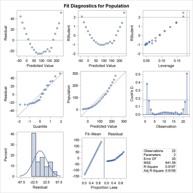
Figure 83.9 shows a plot of residuals versus Year. Again you can see the quadratic pattern that strongly indicates that a quadratic term should be added to the model.

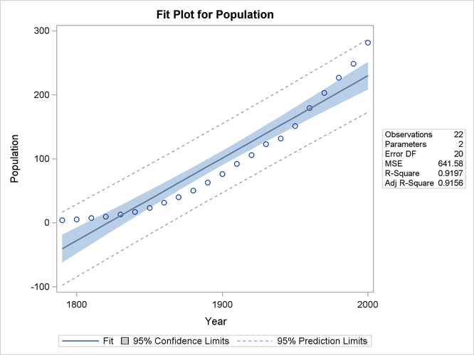
Figure 83.10 shows the FitPlot consisting of a scatter plot of the data overlaid with the regression line, and 95% confidence and prediction limits. Note that this plot also indicates that the model fails to capture the quadratic nature of the data. This plot is produced for models containing a single regressor. You can use the ALPHA= option in the model statement to change the significance level of the confidence band and prediction limits.
These default plots provide strong evidence that the Yearsq needs to be added to the model. You can use the interactive feature of PROC REG to do this by specifying the following statements:
   add YearSq;
   print;
run;
The ADD statement requests that YearSq be added to the model, and the PRINT command causes the model to be refit and displays the ANOVA and parameter estimates
for the new model. The print statement also produces updated ODS graphical displays.
Figure 83.11 displays the ANOVA table and parameter estimates for the new model.
Figure 83.11: ANOVA Table and Parameter Estimates
| Analysis of Variance | |||||
|---|---|---|---|---|---|
| Source | DF | Sum of Squares |
Mean Square |
F Value | Pr > F |
| Model | 2 | 159529 | 79765 | 8864.19 | <.0001 |
| Error | 19 | 170.97193 | 8.99852 | ||
| Corrected Total | 21 | 159700 | |||
| Root MSE | 2.99975 | R-Square | 0.9989 |
|---|---|---|---|
| Dependent Mean | 94.64800 | Adj R-Sq | 0.9988 |
| Coeff Var | 3.16938 |
| Parameter Estimates | |||||
|---|---|---|---|---|---|
| Variable | DF | Parameter Estimate |
Standard Error |
t Value | Pr > |t| |
| Intercept | 1 | 21631 | 639.50181 | 33.82 | <.0001 |
| Year | 1 | -24.04581 | 0.67547 | -35.60 | <.0001 |
| YearSq | 1 | 0.00668 | 0.00017820 | 37.51 | <.0001 |
The overall F statistic is still significant (F = 8864.19, p < 0.0001). The R-square has increased from 0.9197 to 0.9989, indicating that the model now accounts for 99.9% of the variation
in Population. All effects are significant with p < 0.0001 for each effect in the model.
The fitted equation is now
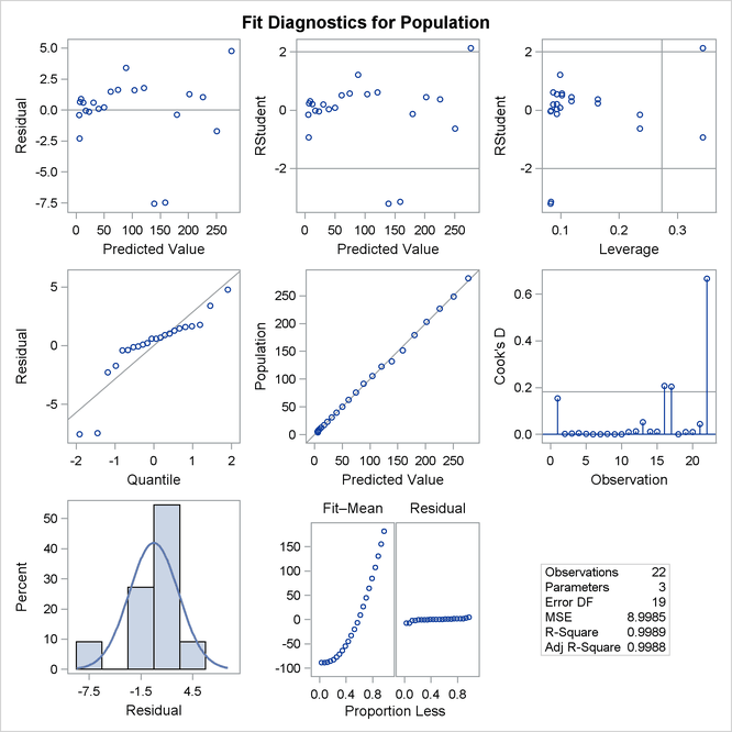
Figure 83.12 show the panel of diagnostics for this quadratic polynomial model. These diagnostics indicate that this model is considerably more successful than the corresponding linear model:
-
The plots of residuals and studentized residuals versus predicted values exhibit no obvious patterns.
-
The points on the plot of the dependent variable versus the predicted values lie along a 45-degree line, indicating that the model successfully predicts the behavior of the dependent variable.
-
The plot of studentized residual versus leverage shows that the years 1790 and 2000 are leverage points with 2000 showing up as an outlier. This is confirmed by the plot of Cook’s D distance versus observation number. This suggests that while the quadratic model fits the current data well, the model might not be quite so successful over a wider range of data. You might want to investigate whether the population trend over the last couple of decades is growing slightly faster than quadratically.
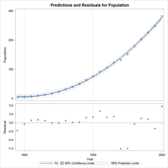
When a model contains more than one regressor, PROC REG does not produce a fit plot. However, when all the regressors in the model are functions of a single variable, it is appropriate to plot predictions and residuals as a function of that variable. You request such plots by using the PLOTS=PREDICTIONS option in the PROC REG statement, as the following code illustrates:
proc reg data=USPopulation plots=predictions(X=Year);
   model Population=Year Yearsq;
quit;

ods graphics off;
Figure 83.13 shows the data, predictions, and residuals by Year. These plots confirm that the quadratic polynomial model successfully model the growth in U.S. population between the years
1780 and 2000.
To complete an analysis of these data, you might want to examine influence statistics and, since the data are essentially time series data, examine the Durbin-Watson statistic.