The REG Procedure
- Overview
-
Getting Started

-
Syntax
-
DetailsMissing ValuesInput Data SetsOutput Data SetsInteractive AnalysisModel-Selection MethodsCriteria Used in Model-Selection MethodsLimitations in Model-Selection MethodsParameter Estimates and Associated StatisticsPredicted and Residual ValuesModels of Less Than Full RankCollinearity DiagnosticsModel Fit and Diagnostic StatisticsInfluence StatisticsReweighting Observations in an AnalysisTesting for HeteroscedasticityTesting for Lack of FitMultivariate TestsAutocorrelation in Time Series DataComputations for Ridge Regression and IPC AnalysisConstruction of Q-Q and P-P PlotsComputational MethodsComputer Resources in Regression AnalysisDisplayed OutputPlot Options Superseded by ODS GraphicsODS Table NamesODS Graphics
-
Examples
- References
This section discusses the INFLUENCE option, which produces several influence statistics, and the PARTIAL option, which produces partial regression leverage plots.
The INFLUENCE option (in the MODEL statement) requests the statistics proposed by Belsley, Kuh, and Welsch (1980) to measure the influence of each observation on the estimates. Influential observations are those that, according to various criteria, appear to have a large influence on the parameter estimates.
Let ![]() be the parameter estimates after deleting the ith observation; let
be the parameter estimates after deleting the ith observation; let ![]() be the variance estimate after deleting the ith observation; let
be the variance estimate after deleting the ith observation; let ![]() be the
be the ![]() matrix without the ith observation; let
matrix without the ith observation; let ![]() be the ith value predicted without using the ith observation; let
be the ith value predicted without using the ith observation; let ![]() be the ith residual; and let
be the ith residual; and let ![]() be the ith diagonal of the projection matrix for
the predictor space, also called the hat matrix:
be the ith diagonal of the projection matrix for
the predictor space, also called the hat matrix:
Belsley, Kuh, and Welsch (1980) propose a cutoff of ![]() , where n is the number of observations used to fit the model and p is the number of parameters in the model. Observations with
, where n is the number of observations used to fit the model and p is the number of parameters in the model. Observations with ![]() values above this cutoff should be investigated.
values above this cutoff should be investigated.
For each observation, PROC REG first displays the residual, the studentized residual (RSTUDENT), and the ![]() .
The studentized residual RSTUDENT differs slightly from STUDENT since the error variance is estimated by
.
The studentized residual RSTUDENT differs slightly from STUDENT since the error variance is estimated by ![]() without the ith observation, not by
without the ith observation, not by ![]() . For example,
. For example,
Observations with RSTUDENT larger than 2 in absolute value might need some attention.
The COVRATIO statistic measures the change in the determinant of the covariance matrix of the estimates by deleting the ith observation:
Belsley, Kuh, and Welsch (1980) suggest that observations with
where p is the number of parameters in the model and n is the number of observations used to fit the model, are worth investigation.
The DFFITS statistic is a scaled measure of the change in the predicted value for the ith observation and
is calculated by deleting the ith observation. A large value indicates that the observation is very influential in its neighborhood of the ![]() space.
space.
Large values of DFFITS indicate influential observations. A general cutoff to consider is 2; a size-adjusted cutoff recommended
by Belsley, Kuh, and Welsch (1980) is ![]() , where n and p are as defined previously.
, where n and p are as defined previously.
The DFFITS statistic is very similar to Cook’s D, defined in the section Predicted and Residual Values.
The DFBETAS statistics are the scaled measures of the change in each parameter estimate and are calculated by deleting the ith observation:
where ![]() is the
is the ![]() element of
element of ![]() .
.
In general, large values of DFBETAS indicate observations that are influential in estimating a given parameter. Belsley, Kuh,
and Welsch (1980) recommend 2 as a general cutoff value to indicate influential observations and ![]() as a size-adjusted cutoff.
as a size-adjusted cutoff.
The following statements use a subset of the data in the population example in the section Polynomial Regression. The INFLUENCE option produces the tables shown in Figure 83.36 and Figure 83.37.
proc reg data=USPopulation;
   where Year <= 1970;
   model Population=Year YearSq / influence;
run;
Figure 83.36: Regression Using the INFLUENCE Option
| Output Statistics | ||||||||
|---|---|---|---|---|---|---|---|---|
| Obs | Residual | RStudent | Hat Diag H |
Cov Ratio |
DFFITS | DFBETAS | ||
| Intercept | Year | YearSq | ||||||
| 1 | -1.1094 | -0.4972 | 0.3865 | 1.8834 | -0.3946 | -0.2842 | 0.2810 | -0.2779 |
| 2 | 0.2691 | 0.1082 | 0.2501 | 1.6147 | 0.0625 | 0.0376 | -0.0370 | 0.0365 |
| 3 | 0.9305 | 0.3561 | 0.1652 | 1.4176 | 0.1584 | 0.0666 | -0.0651 | 0.0636 |
| 4 | 0.7908 | 0.2941 | 0.1184 | 1.3531 | 0.1078 | 0.0182 | -0.0172 | 0.0161 |
| 5 | 0.2110 | 0.0774 | 0.0983 | 1.3444 | 0.0256 | -0.0030 | 0.0033 | -0.0035 |
| 6 | -0.6629 | -0.2431 | 0.0951 | 1.3255 | -0.0788 | 0.0296 | -0.0302 | 0.0307 |
| 7 | -0.8869 | -0.3268 | 0.1009 | 1.3214 | -0.1095 | 0.0609 | -0.0616 | 0.0621 |
| 8 | -0.2501 | -0.0923 | 0.1095 | 1.3605 | -0.0324 | 0.0216 | -0.0217 | 0.0218 |
| 9 | -0.7593 | -0.2820 | 0.1164 | 1.3519 | -0.1023 | 0.0743 | -0.0745 | 0.0747 |
| 10 | -0.5757 | -0.2139 | 0.1190 | 1.3650 | -0.0786 | 0.0586 | -0.0587 | 0.0587 |
| 11 | 0.7938 | 0.2949 | 0.1164 | 1.3499 | 0.1070 | -0.0784 | 0.0783 | -0.0781 |
| 12 | 1.1492 | 0.4265 | 0.1095 | 1.3144 | 0.1496 | -0.1018 | 0.1014 | -0.1009 |
| 13 | 3.1664 | 1.2189 | 0.1009 | 1.0168 | 0.4084 | -0.2357 | 0.2338 | -0.2318 |
| 14 | 1.6746 | 0.6207 | 0.0951 | 1.2430 | 0.2013 | -0.0811 | 0.0798 | -0.0784 |
| 15 | 2.2406 | 0.8407 | 0.0983 | 1.1724 | 0.2776 | -0.0427 | 0.0404 | -0.0380 |
| 16 | -6.6335 | -3.1845 | 0.1184 | 0.2924 | -1.1673 | -0.1531 | 0.1636 | -0.1747 |
| 17 | -6.0147 | -2.8433 | 0.1652 | 0.3989 | -1.2649 | -0.4843 | 0.4958 | -0.5076 |
| 18 | 1.6770 | 0.6847 | 0.2501 | 1.4757 | 0.3954 | 0.2240 | -0.2274 | 0.2308 |
| 19 | 3.9895 | 1.9947 | 0.3865 | 0.9766 | 1.5831 | 1.0902 | -1.1025 | 1.1151 |
Figure 83.37: Residual Statistics
| Sum of Residuals | -5.8175E-11 |
|---|---|
| Sum of Squared Residuals | 123.74557 |
| Predicted Residual SS (PRESS) | 188.54924 |
In Figure 83.36, observations 16, 17, and 19 exceed or are near the cutoff value of 2 for RSTUDENT. None of the observations exceeds the general cutoff of 2 for DFFITS or the DFBETAS, but observations 16, 17, and 19 exceed at least one of the size-adjusted cutoffs for these statistics. Observations 1 and 19 exceed the cutoff for the hat diagonals, and observations 1, 2, 16, 17, and 18 exceed the cutoffs for COVRATIO. Taken together, these statistics indicate that you should look first at observations 16, 17, and 19 and then perhaps investigate the other observations that exceeded a cutoff.
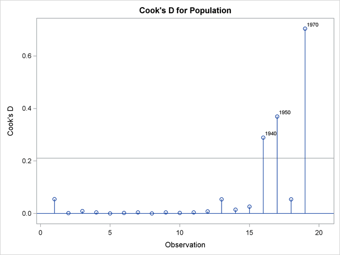
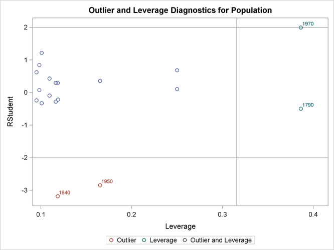
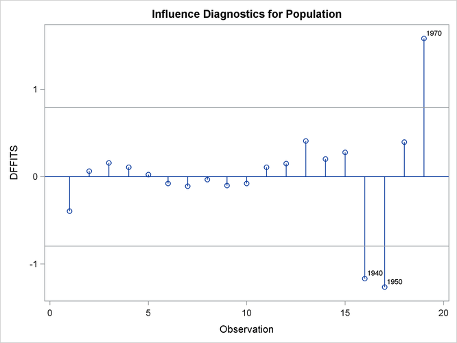
When ODS Graphics is enabled, you can request influence diagnostic plots by using the PLOTS= option in the PROC REG statement as shown in the following statements:
ods graphics on;

proc reg data=USPopulation
      plots(label)=(CooksD RStudentByLeverage DFFITS DFBETAS);
   where Year <= 1970;
   id Year;
   model Population=Year YearSq;
run;

ods graphics off;
The LABEL suboption specified in the PLOTS(LABEL)= option requests that observations that exceed the relevant cutoffs for
the statistics being plotted are labeled. Since Year has been named in an ID statement, the value of Year is used for the labels. The requested plots are shown in Figure 83.38.

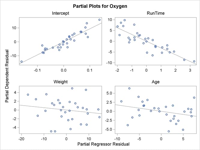
The PARTIAL option in the MODEL statement produces partial regression leverage plots. If ODS Graphics is not enabled, this option requires the use of the LINEPRINTER option in the PROC REG statement. One plot is created for each regressor in the current full model. For example, plots are produced for regressors included by using ADD statements; plots are not produced for interim models in the various model-selection methods but only for the full model. If you use a model-selection method and the final model contains only a subset of the original regressors, the PARTIAL option still produces plots for all regressors in the full model. If ODS Graphics is enabled, these plots are produced as high-resolution graphics, in panels with a maximum of six partial regression leverage plots per panel. Multiple panels are displayed for models with more than six regressors.
For a given regressor, the partial regression leverage plot is the plot of the dependent variable and the regressor after they have been made orthogonal to the other regressors in the model. These can be obtained by plotting the residuals for the dependent variable against the residuals for the selected regressor, where the residuals for the dependent variable are calculated with the selected regressor omitted, and the residuals for the selected regressor are calculated from a model where the selected regressor is regressed on the remaining regressors. A line fit to the points has a slope equal to the parameter estimate in the full model.
When ODS Graphics is not enabled, points in the plot are marked by the number of replicates appearing at one position. The symbol '*' is used if there are 10 or more replicates. If an ID statement is specified, the leftmost nonblank character in the value of the ID variable is used as the plotting symbol.
The PARTIALDATA option in the MODEL statement produces a table that contains the partial regression data that are displayed in the partial regression leverage plots. You can request partial regression data even if you do not requests plots with the PARTIAL option.
The following statements use the fitness data in Example 83.2 with the PARTIAL option and ODS Graphics to produce the partial regression leverage plots. The plots are shown in Figure 83.39.
ods graphics on;

proc reg data=fitness;
   model Oxygen=RunTime Weight Age / partial;
run;

ods graphics off;