The REG Procedure
- Overview
-
Getting Started

-
Syntax
-
DetailsMissing ValuesInput Data SetsOutput Data SetsInteractive AnalysisModel-Selection MethodsCriteria Used in Model-Selection MethodsLimitations in Model-Selection MethodsParameter Estimates and Associated StatisticsPredicted and Residual ValuesModels of Less Than Full RankCollinearity DiagnosticsModel Fit and Diagnostic StatisticsInfluence StatisticsReweighting Observations in an AnalysisTesting for HeteroscedasticityTesting for Lack of FitMultivariate TestsAutocorrelation in Time Series DataComputations for Ridge Regression and IPC AnalysisConstruction of Q-Q and P-P PlotsComputational MethodsComputer Resources in Regression AnalysisDisplayed OutputPlot Options Superseded by ODS GraphicsODS Table NamesODS Graphics
-
Examples
- References
This example features the use of ODS Graphics in the process of building models by using the REG procedure and highlights the use of fit and influence diagnostics.
The Sashelp.Baseball data set contains salary and performance information for Major League Baseball players who played at least one game in both
the 1986 and 1987 seasons, excluding pitchers. The salaries (Sports Illustrated, April 20, 1987) are for the 1987 season and the performance measures are from 1986 (Collier Books, The 1987 Baseball Encyclopedia Update). The following step displays in Output 83.1.1 the variables in the data set:
proc contents varnum data=sashelp.baseball;
   ods select position;
run;
Output 83.1.1: Sashelp.Baseball Data Set
| Variables in Creation Order | ||||
|---|---|---|---|---|
| # | Variable | Type | Len | Label |
| 1 | Name | Char | 18 | Player's Name |
| 2 | Team | Char | 14 | Team at the End of 1986 |
| 3 | nAtBat | Num | 8 | Times at Bat in 1986 |
| 4 | nHits | Num | 8 | Hits in 1986 |
| 5 | nHome | Num | 8 | Home Runs in 1986 |
| 6 | nRuns | Num | 8 | Runs in 1986 |
| 7 | nRBI | Num | 8 | RBIs in 1986 |
| 8 | nBB | Num | 8 | Walks in 1986 |
| 9 | YrMajor | Num | 8 | Years in the Major Leagues |
| 10 | CrAtBat | Num | 8 | Career Times at Bat |
| 11 | CrHits | Num | 8 | Career Hits |
| 12 | CrHome | Num | 8 | Career Home Runs |
| 13 | CrRuns | Num | 8 | Career Runs |
| 14 | CrRbi | Num | 8 | Career RBIs |
| 15 | CrBB | Num | 8 | Career Walks |
| 16 | League | Char | 8 | League at the End of 1986 |
| 17 | Division | Char | 8 | Division at the End of 1986 |
| 18 | Position | Char | 8 | Position(s) in 1986 |
| 19 | nOuts | Num | 8 | Put Outs in 1986 |
| 20 | nAssts | Num | 8 | Assists in 1986 |
| 21 | nError | Num | 8 | Errors in 1986 |
| 22 | Salary | Num | 8 | 1987 Salary in $ Thousands |
| 23 | Div | Char | 16 | League and Division |
| 24 | logSalary | Num | 8 | Log Salary |
Suppose you want to investigate whether you can model the players’ salaries for the 1987 season based on batting statistics for the previous season and lifetime batting performance. Since the variation in salaries is much greater for higher salaries, it is appropriate to apply a log transformation for this analysis. The following statements begin the analysis:
ods graphics on;

proc reg data=sashelp.baseball;
   id name team league;
   model logSalary = nhits nruns nrbi nbb yrmajor crhits;
run;
Output 83.1.2 shows the default output produced by PROC REG. The number of observations table shows that 59 observations are excluded because they have missing values for at least one of the variables used in the analysis. The analysis of variance and parameter estimates tables provide details about the fitted model.
Output 83.1.2: Default Output from PROC REG
| Number of Observations Read | 322 |
|---|---|
| Number of Observations Used | 263 |
| Number of Observations with Missing Values | 59 |
| Analysis of Variance | |||||
|---|---|---|---|---|---|
| Source | DF | Sum of Squares |
Mean Square |
F Value | Pr > F |
| Model | 6 | 121.53052 | 20.25509 | 60.56 | <.0001 |
| Error | 256 | 85.62322 | 0.33447 | ||
| Corrected Total | 262 | 207.15373 | |||
| Root MSE | 0.57833 | R-Square | 0.5867 |
|---|---|---|---|
| Dependent Mean | 5.92722 | Adj R-Sq | 0.5770 |
| Coeff Var | 9.75719 |
| Parameter Estimates | ||||||
|---|---|---|---|---|---|---|
| Variable | Label | DF | Parameter Estimate |
Standard Error |
t Value | Pr > |t| |
| Intercept | Intercept | 1 | 4.14614 | 0.13612 | 30.46 | <.0001 |
| nHits | Hits in 1986 | 1 | 0.00663 | 0.00210 | 3.15 | 0.0018 |
| nRuns | Runs in 1986 | 1 | 0.00019890 | 0.00398 | 0.05 | 0.9602 |
| nRBI | RBIs in 1986 | 1 | 0.00125 | 0.00235 | 0.53 | 0.5947 |
| nBB | Walks in 1986 | 1 | 0.00672 | 0.00239 | 2.81 | 0.0054 |
| YrMajor | Years in the Major Leagues | 1 | 0.07108 | 0.01925 | 3.69 | 0.0003 |
| CrHits | Career Hits | 1 | 0.00023910 | 0.00014571 | 1.64 | 0.1020 |
Before you accept a regression model, it is important to examine influence and fit diagnostics to see whether the model might be unduly influenced by a few observations and whether the data support the assumptions that underlie the linear regression. To facilitate such investigations, you can obtain diagnostic plots by enabling ODS Graphics.
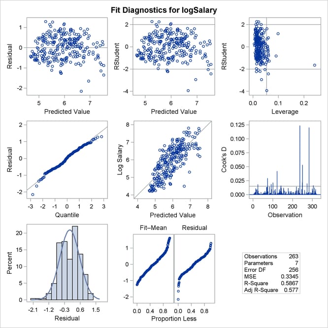
Output 83.1.3 shows a panel of diagnostic plots. The plot of externally studentized residuals (RStudent) by leverage values reveals that there is one observation with very high leverage that might be overly influencing the fit produced. The plot of Cook’s D by observation also indicates two highly influential observations. To investigate further, you can use the PLOTS= option in the PROC REG statement as follows to produce labeled versions of these plots:
proc reg data=sashelp.baseball
         plots(only label)=(RStudentByLeverage CooksD);
   id name team league;
   model logSalary = nhits nruns nrbi nbb yrmajor crhits;
run;
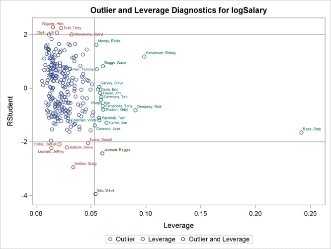
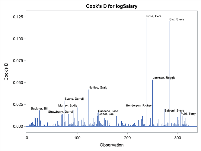
Output 83.1.4 and Output 83.1.5 reveal that Pete Rose is the highly influential observation. You might obtain a better fit to the remaining data if you omit his statistics when building the model.
The following statements use a WHERE statement to omit Pete Rose’s statistics when building the model. An alternative way to do this within PROC REG is to use a REWEIGHT statement. See Reweighting Observations in an Analysis for details about reweighting.
proc reg data=sashelp.baseball
         plots=(RStudentByLeverage(label) residuals(smooth));
   where name^="Rose, Pete";
   id name team league;
   model logSalary = nhits nruns nrbi nbb yrmajor crhits;
run;
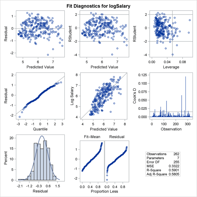
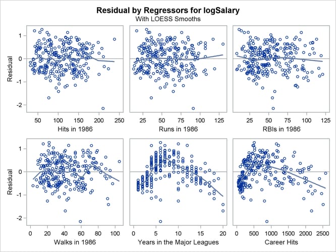
Output 83.1.6 shows the new fit diagnostics panel. You can see that there are still several influential and outlying observations. One possible reason for observing outliers is that the linear model specified is not appropriate to capture the variation in this data. You can often see evidence of an inappropriate model by observing patterns in plots of residuals.
Output 83.1.7 shows plots of the residuals by the regressors in the model. When you specify the RESIDUALS(SMOOTH) suboption of the PLOTS
option in the PROC REG statement, a loess fit is overlaid on each of these plots. You can see the same clear pattern in the residual plots for YrMajor and CrHits. Players near the start of their careers and players near the end of their careers get paid less than the model predicts.
You can address this lack of fit by using polynomials of degree 2 for these two variables as shown in the following statements:
data baseball;
   set sashelp.baseball(where=(name^="Rose, Pete"));
   YrMajor2 = yrmajor*yrmajor;
   CrHits2  = crhits*crhits;
run;

proc reg data=baseball
      plots=(diagnostics(stats=none) RStudentByLeverage(label)
             CooksD(label) Residuals(smooth)
             DFFITS(label) DFBETAS ObservedByPredicted(label));
   id name team league;
   model logSalary = nhits nruns nrbi nbb yrmajor crhits
                     yrmajor2 crhits2;
run;
ods graphics off;
Output 83.1.8 shows the analysis of variance and parameter estimates for this model. Note that the R-square value of 0.787 for this model is considerably larger than the R-square value of 0.587 for the initial model shown in Output 83.1.2.
Output 83.1.8: Output from PROC REG
| Analysis of Variance | |||||
|---|---|---|---|---|---|
| Source | DF | Sum of Squares |
Mean Square |
F Value | Pr > F |
| Model | 8 | 162.73473 | 20.34184 | 117.13 | <.0001 |
| Error | 253 | 43.93712 | 0.17366 | ||
| Corrected Total | 261 | 206.67186 | |||
| Root MSE | 0.41673 | R-Square | 0.7874 |
|---|---|---|---|
| Dependent Mean | 5.92458 | Adj R-Sq | 0.7807 |
| Coeff Var | 7.03393 |
| Parameter Estimates | ||||||
|---|---|---|---|---|---|---|
| Variable | Label | DF | Parameter Estimate |
Standard Error |
t Value | Pr > |t| |
| Intercept | Intercept | 1 | 3.78922 | 0.11581 | 32.72 | <.0001 |
| nHits | Hits in 1986 | 1 | -0.00012753 | 0.00159 | -0.08 | 0.9363 |
| nRuns | Runs in 1986 | 1 | 0.00215 | 0.00288 | 0.75 | 0.4549 |
| nRBI | RBIs in 1986 | 1 | 0.00431 | 0.00172 | 2.51 | 0.0127 |
| nBB | Walks in 1986 | 1 | 0.00501 | 0.00173 | 2.90 | 0.0040 |
| YrMajor | Years in the Major Leagues | 1 | 0.23908 | 0.03443 | 6.94 | <.0001 |
| CrHits | Career Hits | 1 | 0.00170 | 0.00027562 | 6.18 | <.0001 |
| YrMajor2 | 1 | -0.01440 | 0.00165 | -8.73 | <.0001 | |
| CrHits2 | 1 | -3.31739E-7 | 1.001272E-7 | -3.31 | 0.0011 | |
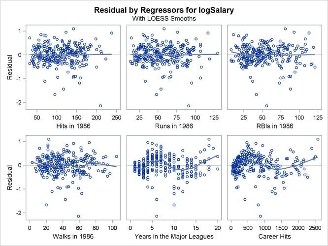
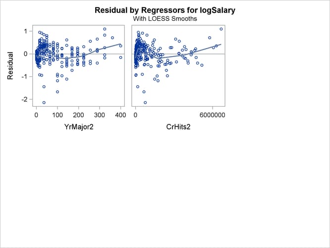
The plots of residuals by regressors in Output 83.1.9 and Output 83.1.10 show that the strong pattern in the plots for CrMajors and CrHits has been reduced, although there is still some indication of a pattern remaining in these residuals. This suggests that a
quadratic function might be insufficient to capture dependence of salary on these regressors.
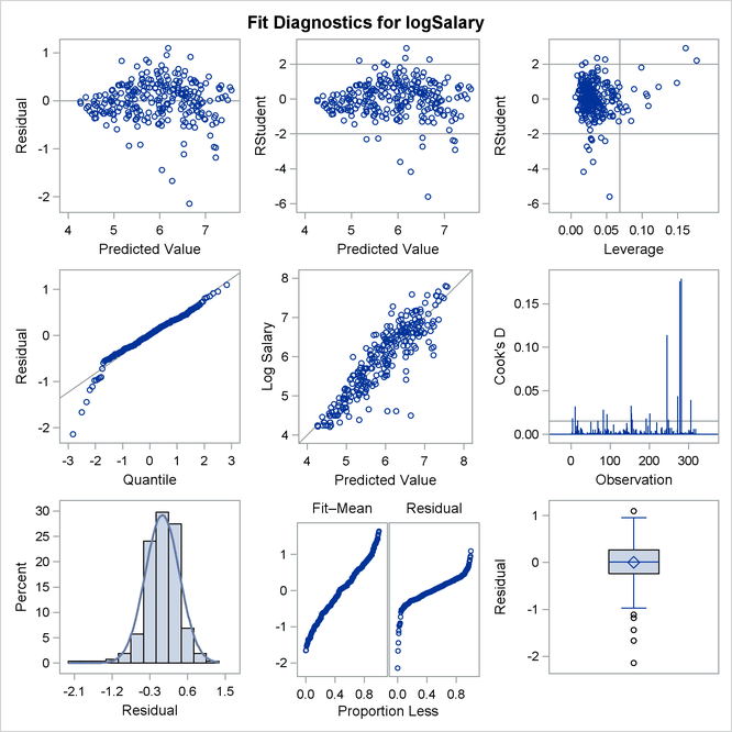
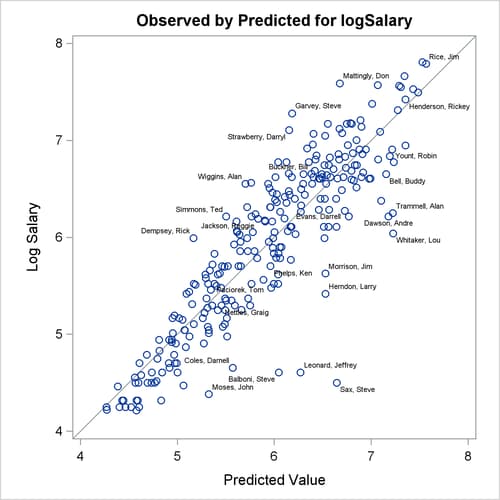
Output 83.1.11 show the diagnostics plots; three of the plots, with points of interest labeled, are shown individually in Output 83.1.12, Output 83.1.13, and Output 83.1.14. The STATS=NONE suboption specified in the PLOTS=DIAGNOSTICS option replaces the inset of statistics with a box plot of the residuals in the fit diagnostics panel. The observed by predicted value plot reveals a reasonably successful model for explaining the variation in salary for most of the players. However, the model tends to overpredict the salaries of several players near the lower end of the salary range. This bias can also be seen in the distribution of the residuals that you can see in the histogram, Q-Q plot, and box plot in Output 83.1.11.
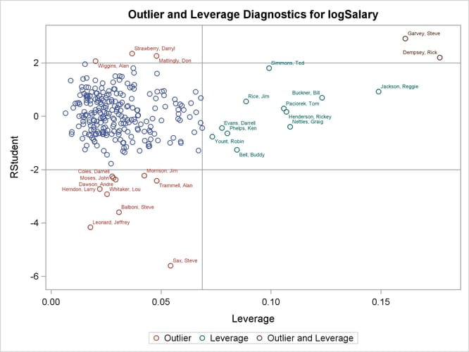
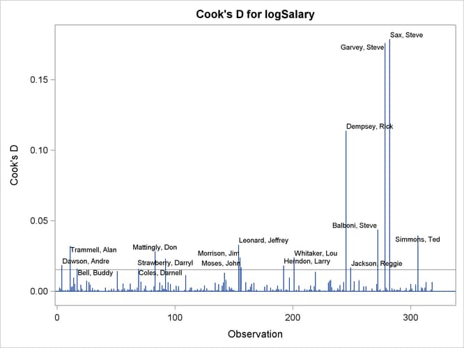
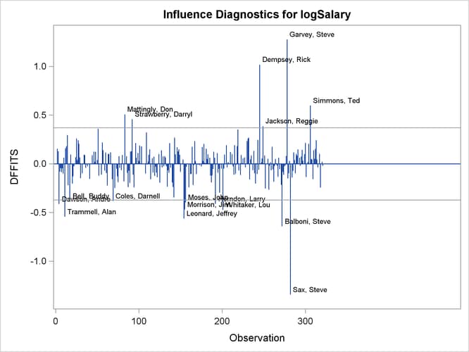
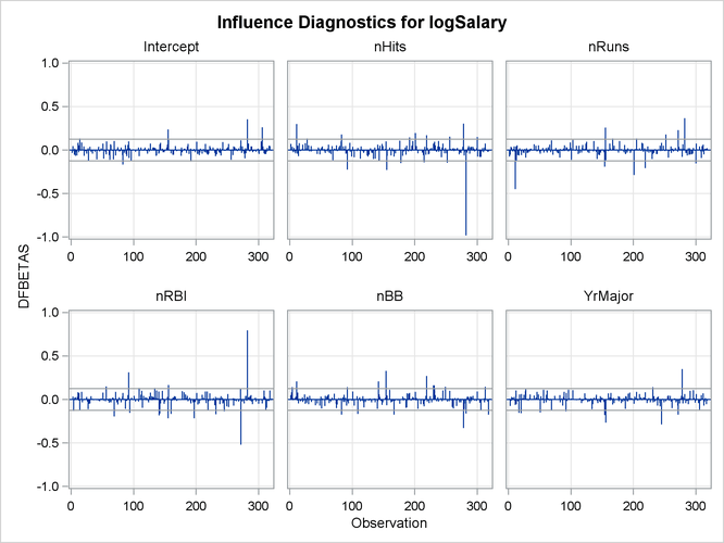
The RStudent by leverage plot in Output 83.1.12 and the Cook’s D plot in Output 83.1.14 show that there are still a number of influential observations. By specifying the DFFITS and DFBETAS suboptions of the PLOTS= option, you obtain additional influence diagnostics plots shown in Output 83.1.15 and Output 83.1.16. See Influence Statistics for details about the interpretation DFFITS and DFBETAS statistics.
You can continue this analysis by investigating how the influential observations identified in the various influence plots affect the fit. You can also use PROC ROBUSTREG to obtain a fit that is resistant to the presence of high leverage points and outliers.