The REG Procedure
- Overview
-
Getting Started

-
Syntax
-
DetailsMissing ValuesInput Data SetsOutput Data SetsInteractive AnalysisModel-Selection MethodsCriteria Used in Model-Selection MethodsLimitations in Model-Selection MethodsParameter Estimates and Associated StatisticsPredicted and Residual ValuesModels of Less Than Full RankCollinearity DiagnosticsModel Fit and Diagnostic StatisticsInfluence StatisticsReweighting Observations in an AnalysisTesting for HeteroscedasticityTesting for Lack of FitMultivariate TestsAutocorrelation in Time Series DataComputations for Ridge Regression and IPC AnalysisConstruction of Q-Q and P-P PlotsComputational MethodsComputer Resources in Regression AnalysisDisplayed OutputPlot Options Superseded by ODS GraphicsODS Table NamesODS Graphics
-
Examples
- References
At times it is desirable to have independent variables in the model that are qualitative rather than quantitative. This is easily handled in a regression framework. Regression uses qualitative variables to distinguish between populations. There are two main advantages of fitting both populations in one model. You gain the ability to test for different slopes or intercepts in the populations, and more degrees of freedom are available for the analysis.
Regression with qualitative variables is different from analysis of variance and analysis of covariance. Analysis of variance uses qualitative independent variables only. Analysis of covariance uses quantitative variables in addition to the qualitative variables in order to account for correlation in the data and reduce MSE; however, the quantitative variables are not of primary interest and merely improve the precision of the analysis.
Consider the case where ![]() is the dependent variable,
is the dependent variable, ![]() is a quantitative variable,
is a quantitative variable, ![]() is a qualitative variable taking on values 0 or 1, and
is a qualitative variable taking on values 0 or 1, and ![]() is the interaction. The variable
is the interaction. The variable ![]() is called a dummy, binary, or indicator variable. With values 0 or 1, it distinguishes between two populations. The model
is of the form
is called a dummy, binary, or indicator variable. With values 0 or 1, it distinguishes between two populations. The model
is of the form
for the observations ![]() . The parameters to be estimated are
. The parameters to be estimated are ![]() ,
, ![]() ,
, ![]() , and
, and ![]() . The number of dummy variables used is one less than the number of qualitative levels. This yields a nonsingular
. The number of dummy variables used is one less than the number of qualitative levels. This yields a nonsingular ![]() matrix. See Chapter 10 of Neter, Wasserman, and Kutner (1990) for more details.
matrix. See Chapter 10 of Neter, Wasserman, and Kutner (1990) for more details.
An example from Neter, Wasserman, and Kutner (1990) follows. An economist is investigating the relationship between the size of an insurance firm and the speed at which it implements new insurance innovations. He believes that the type of firm might affect this relationship and suspects that there might be some interaction between the size and type of firm. The dummy variable in the model enables the two firms to have different intercepts. The interaction term enables the firms to have different slopes as well.
In this study, ![]() is the number of months from the time the first firm implemented the innovation to the time it was implemented by the ith firm. The variable
is the number of months from the time the first firm implemented the innovation to the time it was implemented by the ith firm. The variable ![]() is the size of the firm, measured in total assets of the firm. The variable
is the size of the firm, measured in total assets of the firm. The variable ![]() denotes the firm type; it is 0 if the firm is a mutual fund company and 1 if the firm is a stock company. The dummy variable
enables each firm type to have a different intercept and slope.
denotes the firm type; it is 0 if the firm is a mutual fund company and 1 if the firm is a stock company. The dummy variable
enables each firm type to have a different intercept and slope.
The previous model can be broken down into a model for each firm type by plugging in the values for ![]() . If
. If ![]() , the model is
, the model is
This is the model for a mutual company. If ![]() , the model for a stock firm is
, the model for a stock firm is
This model has intercept ![]() and slope
and slope ![]() .
.
The data[35] follow. Note that the interaction term is created in the DATA step since polynomial effects such as size*type are not allowed in the MODEL statement in the REG procedure.
title 'Regression with Quantitative and Qualitative Variables';
data insurance;
   input time size type @@;
   sizetype=size*type;
   datalines;
17 151 0   26  92 0   21 175 0   30  31 0   22 104 0   0  277 0   12 210 0
19 120 0    4 290 0   16 238 0   28 164 1   15 272 1   11 295 1   38  68 1
31  85 1   21 224 1   20 166 1   13 305 1   30 124 1   14 246 1
;
The following statements begin the analysis and produce the ANOVA table in Output 83.4.1:
proc reg data=insurance;
   model time = size type sizetype;
run;
Output 83.4.1: ANOVA Table and Parameter Estimates
| Regression with Quantitative and Qualitative Variables |
| Analysis of Variance | |||||
|---|---|---|---|---|---|
| Source | DF | Sum of Squares |
Mean Square |
F Value | Pr > F |
| Model | 3 | 1504.41904 | 501.47301 | 45.49 | <.0001 |
| Error | 16 | 176.38096 | 11.02381 | ||
| Corrected Total | 19 | 1680.80000 | |||
| Root MSE | 3.32021 | R-Square | 0.8951 |
|---|---|---|---|
| Dependent Mean | 19.40000 | Adj R-Sq | 0.8754 |
| Coeff Var | 17.11450 |
| Parameter Estimates | |||||
|---|---|---|---|---|---|
| Variable | DF | Parameter Estimate |
Standard Error |
t Value | Pr > |t| |
| Intercept | 1 | 33.83837 | 2.44065 | 13.86 | <.0001 |
| size | 1 | -0.10153 | 0.01305 | -7.78 | <.0001 |
| type | 1 | 8.13125 | 3.65405 | 2.23 | 0.0408 |
| sizetype | 1 | -0.00041714 | 0.01833 | -0.02 | 0.9821 |
The overall F statistic is significant (F = 45.490, p < 0.0001). The interaction term is not significant (t = –0.023, p = 0.9821). Hence, this term should be removed and the model refitted, as shown in the following statements:
   delete sizetype;
   print;
run;
The DELETE statement removes the interaction term (sizetype) from the model. The new ANOVA and parameter estimates tables are shown in Output 83.4.2.
Output 83.4.2: ANOVA Table and Parameter Estimates
| Analysis of Variance | |||||
|---|---|---|---|---|---|
| Source | DF | Sum of Squares |
Mean Square |
F Value | Pr > F |
| Model | 2 | 1504.41333 | 752.20667 | 72.50 | <.0001 |
| Error | 17 | 176.38667 | 10.37569 | ||
| Corrected Total | 19 | 1680.80000 | |||
| Root MSE | 3.22113 | R-Square | 0.8951 |
|---|---|---|---|
| Dependent Mean | 19.40000 | Adj R-Sq | 0.8827 |
| Coeff Var | 16.60377 |
| Parameter Estimates | |||||
|---|---|---|---|---|---|
| Variable | DF | Parameter Estimate |
Standard Error |
t Value | Pr > |t| |
| Intercept | 1 | 33.87407 | 1.81386 | 18.68 | <.0001 |
| size | 1 | -0.10174 | 0.00889 | -11.44 | <.0001 |
| type | 1 | 8.05547 | 1.45911 | 5.52 | <.0001 |
The overall F statistic is still significant (F = 72.497, p < 0.0001). The intercept and the coefficients associated with size and type are significantly different from zero (t = 18.675, p < 0.0001; t = –11.443, p < 0.0001; t = 5.521, p < 0.0001, respectively). Notice that the R square did not change with the omission of the interaction term.
The fitted model is
The fitted model for a mutual fund company (![]() ) is
) is
and the fitted model for a stock company (![]() ) is
) is
So the two models have different intercepts but the same slope.
The following statements first use an OUTPUT statement to save the residuals and predicted values from the new model in the OUT= data set. Next PROC SGPLOT is used to produce Output 83.4.3, which plots residuals versus predicted values. The firm type is used as the plot symbol; this can be useful in determining if the firm types have different residual patterns.
   output out=out r=r p=p;
run;

proc sgplot data=out;
   scatter x=p y=r / markerchar=type group=type;
run;
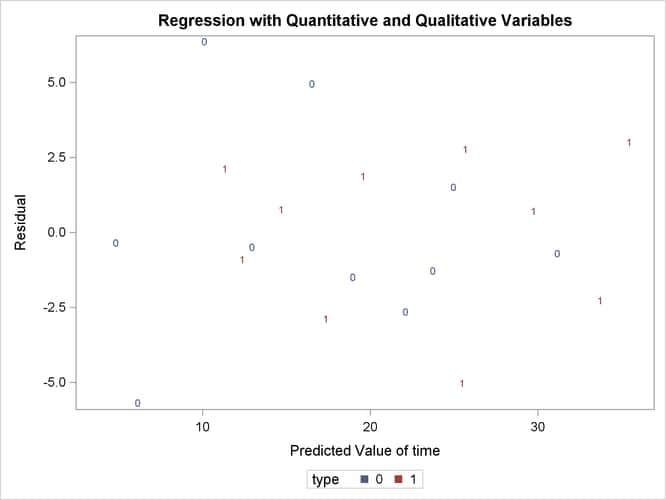
The residuals show no major trend. Neither firm type by itself shows a trend either. This indicates that the model is satisfactory.
The following statements produce the plot of the predicted values versus size that appears in Output 83.4.4, where the firm type is again used as the plotting symbol:
proc sgplot data=out;
   scatter x=size y=p / markerchar=type group=type;
run;
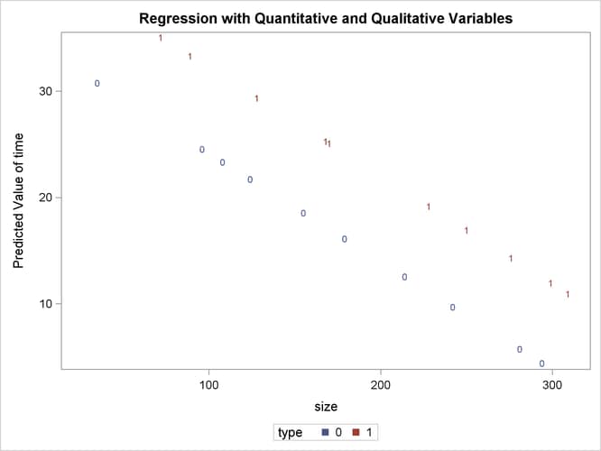
The different intercepts are very evident in this plot.
[35] From Neter, J., et al., Applied Linear Statistical Models, Third Edition, Copyright (c) 1990, Richard D. Irwin. Reprinted with permission of The McGraw-Hill Companies.