The GLM Procedure

If you fit several dependent variables to the same effects, you might want to make joint tests involving parameters of several dependent variables. Suppose you have dependent variables, parameters for each dependent variable, and observations. The models can be collected into one equation:

where is , is , is , and is . Each of the models can be estimated and tested separately. However, you might also want to consider the joint distribution and test the models simultaneously.

For multivariate tests, you need to make some assumptions about the errors. With dependent variables, there are errors that are independent across observations but not across dependent variables. Assume

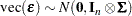where vec strings out by rows, denotes Kronecker product multiplication, and is . can be estimated by

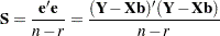where , is the rank of the matrix, and is the matrix of residuals.

If is scaled to unit diagonals, the values in are called partial correlations of the Ys adjusting for the Xs. This matrix can be displayed by PROC GLM if PRINTE is specified as a MANOVA option.

The multivariate general linear hypothesis is written

You can form hypotheses for linear combinations across columns, as well as across rows of .

The MANOVA statement of the GLM procedure tests special cases where corresponds to Type I, Type II, Type III, or Type IV tests, and is the identity matrix. These tests are joint tests that the given type of hypothesis holds for all dependent variables in the model, and they are often sufficient to test all hypotheses of interest.

Finally, when these special cases are not appropriate, you can specify your own and matrices by using the CONTRAST statement before the MANOVA statement and the M= specification in the MANOVA statement, respectively. Another alternative is to use a REPEATED statement, which automatically generates a variety of matrices useful in repeated measures analysis of variance. See the section REPEATED Statement and the section Repeated Measures Analysis of Variance for more information.

One useful way to think of a MANOVA analysis with an matrix other than the identity is as an analysis of a set of transformed variables defined by the columns of the matrix. You should note, however, that PROC GLM always displays the matrix in such a way that the transformed variables are defined by the rows, not the columns, of the displayed matrix.

All multivariate tests carried out by the GLM procedure first construct the matrices and corresponding to the numerator and denominator, respectively, of a univariate test:

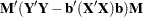The diagonal elements of and correspond to the hypothesis and error SS for univariate tests. When the matrix is the identity matrix (the default), these tests are for the original dependent variables on the left side of the MODEL statement. When an matrix other than the identity is specified, the tests are for transformed variables defined by the columns of the matrix. These tests can be studied by requesting the SUMMARY option, which produces univariate analyses for each original or transformed variable.

Four multivariate test statistics, all functions of the eigenvalues of (or ), are constructed:

• Wilks’ lambda = det/det

• Pillai’s trace = trace

• Hotelling-Lawley trace = trace

• Roy’s greatest root = , largest eigenvalue of

By default, all four are reported with p-values based on approximations, as discussed in the "Multivariate Tests" section in Chapter 4, Introduction to Regression Procedures. Alternatively, if you specify MSTAT=EXACT in the associated MANOVA or REPEATED statement, p-values for three of the four tests are computed exactly (Wilks’ lambda, the Hotelling-Lawley trace, and Roy’s greatest root), and the p-values for the fourth (Pillai’s trace) are based on an approximation that is more accurate than the default. See the "Multivariate Tests" section in Chapter 4, Introduction to Regression Procedures, for more details on the exact calculations.