The UNIVARIATE Procedure

PPPLOT Statement

Distribution Options
General Options
Dictionary of Options

PPPLOT <variables> < / options> ;

The PPPLOT statement creates a probability-probability plot (also referred to as a P-P plot or percent plot), which compares the empirical cumulative distribution function (ecdf) of a variable with a specified theoretical cumulative distribution function such as the normal. If the two distributions match, the points on the plot form a linear pattern that passes through the origin and has unit slope. Thus, you can use a P-P plot to determine how well a theoretical distribution models a set of measurements.

You can specify one of the following theoretical distributions with the PPPLOT statement:

beta
exponential
gamma
Gumbel
generalized Pareto
inverse Gaussian
lognormal
normal
power function
Rayleigh
Weibull

Note: Probability-probability plots should not be confused with probability plots, which compare a set of ordered measurements with percentiles from a specified distribution. You can create probability plots with the PROBPLOT statement.

You can use any number of PPPLOT statements in the UNIVARIATE procedure. The components of the PPPLOT statement are as follows.

variables

are the process variables for which P-P plots are created. If you specify a VAR statement, the variables must also be listed in the VAR statement. Otherwise, the variables can be any numeric variables in the input data set. If you do not specify a list of variables, then by default, the procedure creates a P-P plot for each variable listed in the VAR statement or for each numeric variable in the input data set if you do not specify a VAR statement. For example, if data set measures contains two numeric variables, length and width, the following two PPPLOT statements each produce a P-P plot for each of those variables:

proc univariate data=measures;
   var length width;
   ppplot;
run;

proc univariate data=measures;
   ppplot length width;
run;

options

specify the theoretical distribution for the plot or add features to the plot. If you specify more than one variable, the options apply equally to each variable. Specify all options after the slash (/) in the PPPLOT statement. You can specify only one option that names a distribution, but you can specify any number of other options. By default, the procedure produces a P-P plot based on the normal distribution.

In the following example, the NORMAL, MU=, and SIGMA= options request a P-P plot based on the normal distribution with mean 10 and standard deviation 0.3. The SQUARE option displays the plot in a square frame, and the CTEXT= option specifies the text color.

proc univariate data=measures;
   ppplot length width / normal(mu=10 sigma=0.3)
                         square
                         ctext=blue;
run;

Table 4.15 through Table 4.17 list the PPPLOT options by function. For complete descriptions, see the sections Dictionary of Options and Dictionary of Common Options. Options can be any of the following:

primary options
secondary options
general options

Distribution Options

Table 4.15 summarizes the options for requesting a specific theoretical distribution.

Table 4.15: Options for Specifying the Theoretical Distribution

Option	Description
BETA(beta-options)	specifies beta P-P plot
EXPONENTIAL(exponential-options)	specifies exponential P-P plot
GAMMA(gamma-options)	specifies gamma P-P plot
GUMBEL(Gumbel-options)	specifies Gumbel P-P plot
PARETO(Pareto-options)	specifies generalized Pareto P-P plot
IGAUSS(iGauss-options)	specifies inverse Gaussian P-P plot
LOGNORMAL(lognormal-options)	specifies lognormal P-P plot
NORMAL(normal-options)	specifies normal P-P plot
POWER(power-options)	specifies power function P-P plot
RAYLEIGH(Rayleigh-options)	specifies Rayleigh P-P plot
WEIBULL(Weibull-options)	specifies Weibull P-P plot

Table 4.16 summarizes options that specify distribution parameters and control the display of the diagonal distribution reference line. Specify these options in parentheses after the distribution option. For example, the following statements use the NORMAL option to request a normal P-P plot:

proc univariate data=measures;
   ppplot length / normal(mu=10 sigma=0.3 color=red);
run;

The MU= and SIGMA= normal-options specify $\mu$ and $\sigma$ for the normal distribution, and the COLOR= normal-option specifies the color for the line.

Table 4.16: Secondary Distribution Reference Line Options

Option	Description
Options Used with All Distributions
COLOR=	specifies color of distribution reference line
L=	specifies line type of distribution reference line
NOLINE	suppresses the distribution reference line
W=	specifies width of distribution reference line
Beta-Options
ALPHA=	specifies shape parameter $\alpha$
BETA=	specifies shape parameter $\beta$
SIGMA=	specifies scale parameter $\sigma$
THETA=	specifies lower threshold parameter $\theta$
Exponential-Options
SIGMA=	specifies scale parameter $\sigma$
THETA=	specifies threshold parameter $\theta$
Gamma-Options
ALPHA=	specifies shape parameter $\alpha$
ALPHADELTA=	specifies change in successive estimates of $\alpha$ at which the Newton-Raphson approximation of $\hat{\alpha }$ terminates
ALPHAINITIAL=	specifies initial value for $\alpha$ in the Newton-Raphson approximation of $\hat{\alpha }$
MAXITER=	specifies maximum number of iterations in the Newton-Raphson approximation of $\hat{\alpha }$
SIGMA=	specifies scale parameter $\sigma$
THETA=	specifies threshold parameter $\theta$
Gumbel-Options
MU=	specifies location parameter $\mu$
SIGMA=	specifies scale parameter $\sigma$
IGauss-Options
LAMBDA=	specifies shape parameter $\lambda$
MU=	specifies mean $\mu$
Lognormal-Options
SIGMA=	specifies shape parameter $\sigma$
THETA=	specifies threshold parameter $\theta$
ZETA=	specifies scale parameter $\zeta$
Normal-Options
MU=	specifies mean $\mu$
SIGMA=	specifies standard deviation $\sigma$
Pareto-Options
ALPHA=	specifies shape parameter $\alpha$
SIGMA=	specifies scale parameter $\sigma$
THETA=	specifies threshold parameter $\theta$
Power-Options
ALPHA=	specifies shape parameter $\alpha$
SIGMA=	specifies scale parameter $\sigma$
THETA=	specifies threshold parameter $\theta$
Rayleigh-Options
SIGMA=	specifies scale parameter $\sigma$
THETA=	specifies threshold parameter $\theta$
Weibull-Options
C=	specifies shape parameter
ITPRINT	requests table of iteration history and optimizer details
MAXITER=	specifies maximum number of iterations in the Newton-Raphson approximation of $\hat{c}$
SIGMA=	specifies scale parameter $\sigma$
THETA=	specifies threshold parameter $\theta$

General Options

Table 4.17 lists options that control the appearance of the plots. For complete descriptions, see the sections Dictionary of Options and Dictionary of Common Options.

Table 4.17: General Graphics Options

Option	Description
General Graphics Options
HREF=	specifies reference lines perpendicular to the horizontal axis
HREFLABELS=	specifies line labels for HREF= lines
HREFLABPOS=	specifies position for HREF= line labels
NOHLABEL	suppresses label for horizontal axis
NOVLABEL	suppresses label for vertical axis
NOVTICK	suppresses tick marks and tick mark labels for vertical axis
SQUARE	displays P-P plot in square format
VAXISLABEL=	specifies label for vertical axis
VREF=	specifies reference lines perpendicular to the vertical axis
VREFLABELS=	specifies line labels for VREF= lines
VREFLABPOS=	specifies position for VREF= line labels
Options for Traditional Graphics Output
ANNOTATE=	provides an annotate data set
CAXIS=	specifies color for axis
CFRAME=	specifies color for frame
CHREF=	specifies colors for HREF= lines
CTEXT=	specifies color for text
CVREF=	specifies colors for VREF= lines
DESCRIPTION=	specifies description for plot in graphics catalog
FONT=	specifies software font for text
HAXIS=	specifies AXIS statement for horizontal axis
HEIGHT=	specifies height of text used outside framed areas
HMINOR=	specifies number of minor tick marks on horizontal axis
INFONT=	specifies software font for text inside framed areas
INHEIGHT=	specifies height of text inside framed areas
LHREF=	specifies line types for HREF= lines
LVREF=	specifies line types for VREF= lines
NAME=	specifies name for plot in graphics catalog
NOFRAME	suppresses frame around plotting area
TURNVLABELS	turns and vertically strings out characters in labels for vertical axis
VAXIS=	specifies AXIS statement for vertical axis
VMINOR=	specifies number of minor tick marks on vertical axis
WAXIS=	specifies line thickness for axes and frame
Options for ODS Graphics Output
ODSFOOTNOTE=	specifies footnote displayed on plot
ODSFOOTNOTE2=	specifies secondary footnote displayed on plot
ODSTITLE=	specifies title displayed on plot
ODSTITLE2=	specifies secondary title displayed on plot
OVERLAY	overlays plots for different class levels (ODS Graphics only)
Options for Comparative Plots
ANNOKEY	applies annotation requested in ANNOTATE= data set to key cell only
CFRAMESIDE=	specifies color for filling row label frames
CFRAMETOP=	specifies color for filling column label frames
CPROP=	specifies color for proportion of frequency bar
CTEXTSIDE=	specifies color for row labels
CTEXTTOP=	specifies color for column labels
INTERTILE=	specifies distance between tiles in comparative plot
NCOLS=	specifies number of columns in comparative plot
NROWS=	specifies number of rows in comparative plot
Miscellaneous Options
CONTENTS=	specifies table of contents entry for P-P plot grouping

Dictionary of Options

The following entries provide detailed descriptions of options for the PPPLOT statement. See the section Dictionary of Common Options for detailed descriptions of options common to all plot statements.

ALPHA=value

specifies the shape parameter $\alpha$ $(\alpha >0)$ for P-P plots requested with the BETA, GAMMA, PARETO and POWER options.

BETA<(beta-options)>

creates a beta P-P plot. To create the plot, the nonmissing observations are ordered from smallest to largest:

$x_{(1)} \leq x_{(2)} \leq \cdots \leq x_{(n)}$

The -coordinate of the th point is the empirical cdf value $\frac{i}{n}$ . The -coordinate is the theoretical beta cdf value

$B_{\alpha \beta }\left(\frac{x_{(i)}-\theta }{\sigma }\right) = \int _{\theta }^{x_{(i)}} \frac{(t-\theta )^{\alpha -1}(\theta +\sigma -t)^{\beta -1} }{B(\alpha ,\beta ) \sigma ^{(\alpha +\beta -1)} } dt$

where $B_{\alpha \beta }(\cdot )$ is the normalized incomplete beta function, 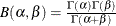$B(\alpha ,\beta ) = \frac{\Gamma (\alpha )\Gamma (\beta )}{\Gamma (\alpha +\beta )}$ , and

$\theta =$ lower threshold parameter
$\sigma =$ scale parameter $(\sigma >0)$
$\alpha =$ first shape parameter $(\alpha >0)$
$\beta =$ second shape parameter $(\beta >0)$

You can specify $\alpha$ , $\beta$ , $\sigma$ , and $\theta$ with the ALPHA=, BETA=, SIGMA=, and THETA= beta-options, as illustrated in the following example:

proc univariate data=measures;
   ppplot width / beta(theta=1 sigma=2 alpha=3 beta=4);
run;

If you do not specify values for these parameters, then by default, $\theta =0$ , $\sigma =1$ , and maximum likelihood estimates are calculated for $\alpha$ and $\beta$ .

IMPORTANT: If the default unit interval (0,1) does not adequately describe the range of your data, then you should specify THETA= $\theta$ and SIGMA= $\sigma$ so that your data fall in the interval $(\theta , \theta +\sigma )$ .

If the data are beta distributed with parameters $\alpha$ , $\beta$ , $\sigma$ , and $\theta$ , then the points on the plot for ALPHA= $\alpha$ , BETA= $\beta$ , SIGMA= $\sigma$ , and THETA= $\theta$ tend to fall on or near the diagonal line , which is displayed by default. Agreement between the diagonal line and the point pattern is evidence that the specified beta distribution is a good fit. You can specify the SCALE= option as an alias for the SIGMA= option and the THRESHOLD= option as an alias for the THETA= option.

BETA=value

specifies the shape parameter $\beta$ $(\beta >0)$ for P-P plots requested with the BETA distribution option. See the preceding entry for the BETA distribution option for an example.

C=value

specifies the shape parameter for P-P plots requested with the WEIBULL option. See the entry for the WEIBULL option for examples.

EXPONENTIAL<(exponential-options)> EXP<(exponential-options)>

creates an exponential P-P plot. To create the plot, the nonmissing observations are ordered from smallest to largest:

$x_{(1)} \leq x_{(2)} \leq \cdots \leq x_{(n)}$

The -coordinate of the th point is the empirical cdf value $\frac{i}{n}$ . The -coordinate is the theoretical exponential cdf value

$F(x_{(i)}) = 1-\exp \left(-\frac{x_{(i)}-\theta }{\sigma }\right)$

where

$\theta =$ threshold parameter
$\sigma =$ scale parameter $(\sigma >0)$

You can specify $\sigma$ and $\theta$ with the SIGMA= and THETA= exponential-options, as illustrated in the following example:

proc univariate data=measures;
   ppplot width / exponential(theta=1 sigma=2);
run;

If you do not specify values for these parameters, then by default, $\theta =0$ and a maximum likelihood estimate is calculated for $\sigma$ .

IMPORTANT: Your data must be greater than or equal to the lower threshold $\theta$ . If the default $\theta =0$ is not an adequate lower bound for your data, specify $\theta$ with the THETA= option.

If the data are exponentially distributed with parameters $\sigma$ and $\theta$ , the points on the plot for SIGMA= $\sigma$ and THETA= $\theta$ tend to fall on or near the diagonal line , which is displayed by default. Agreement between the diagonal line and the point pattern is evidence that the specified exponential distribution is a good fit. You can specify the SCALE= option as an alias for the SIGMA= option and the THRESHOLD= option as an alias for the THETA= option.

GAMMA<(gamma-options)>

creates a gamma P-P plot. To create the plot, the nonmissing observations are ordered from smallest to largest:

$x_{(1)} \leq x_{(2)} \leq \cdots \leq x_{(n)}$

The -coordinate of the th point is the empirical cdf value $\frac{i}{n}$ . The -coordinate is the theoretical gamma cdf value

$G_{\alpha }\left(\frac{x_{(i)}-\theta }{\sigma }\right) = \int _{\theta }^{x_{(i)}} \frac{1}{\sigma \Gamma (\alpha )} \left(\frac{t-\theta }{\sigma }\right)^{\alpha -1} \exp \left(-\frac{t-\theta }{\sigma }\right) dt$

where $G_{\alpha }(\cdot )$ is the normalized incomplete gamma function and

$\theta =$ threshold parameter
$\sigma =$ scale parameter $(\sigma >0)$
$\alpha =$ shape parameter $(\alpha >0)$

You can specify $\alpha$ , $\sigma$ , and $\theta$ with the ALPHA=, SIGMA=, and THETA= gamma-options, as illustrated in the following example:

proc univariate data=measures;
   ppplot width / gamma(alpha=1 sigma=2 theta=3);
run;

If you do not specify values for these parameters, then by default, $\theta =0$ and maximum likelihood estimates are calculated for $\alpha$ and $\sigma$ .

If the data are gamma distributed with parameters $\alpha$ , $\sigma$ , and $\theta$ , the points on the plot for ALPHA= $\alpha$ , SIGMA= $\sigma$ , and THETA= $\theta$ tend to fall on or near the diagonal line , which is displayed by default. Agreement between the diagonal line and the point pattern is evidence that the specified gamma distribution is a good fit. You can specify the SHAPE= option as an alias for the ALPHA= option, the SCALE= option as an alias for the SIGMA= option, and the THRESHOLD= option as an alias for the THETA= option.

GUMBEL<(Gumbel-options)>

creates a Gumbel P-P plot. To create the plot, the nonmissing observations are ordered from smallest to largest:

$x_{(1)} \leq x_{(2)} \leq \cdots \leq x_{(n)}$

The -coordinate of the th point is the empirical cdf value $\frac{i}{n}$ . The -coordinate is the theoretical Gumbel cdf value

$F\left(x_{(i)}\right) = \exp (-e^{-(x_{(i)}-\mu )/\sigma })$

where

$\mu =$ location parameter
$\sigma =$ scale parameter $(\sigma >0)$

You can specify $\mu$ and $\sigma$ with the MU= and SIGMA= Gumbel-options, as illustrated in the following example:

proc univariate data=measures;
   ppplot width / gumbel(mu=1 sigma=2);
run;

If you do not specify values for these parameters, then by default, the maximum likelihood estimates are calculated for $\mu$ and $\sigma$ .

If the data are Gumbel distributed with parameters $\mu$ and $\sigma$ , the points on the plot for MU= $\mu$ and SIGMA= $\sigma$ tend to fall on or near the diagonal line , which is displayed by default. Agreement between the diagonal line and the point pattern is evidence that the specified Gumbel distribution is a good fit.

IGAUSS<(iGauss-options)>

creates an inverse Gaussian P-P plot. To create the plot, the nonmissing observations are ordered from smallest to largest:

$x_{(1)} \leq x_{(2)} \leq \cdots \leq x_{(n)}$

The -coordinate of the th point is the empirical cdf value $\frac{i}{n}$ . The -coordinate is the theoretical inverse Gaussian cdf value

$F(x_{(i)}) = \Phi \left\{ \sqrt {\frac{\lambda }{x_{(i)}}} \left( \frac{x_{(i)}}{\mu }-1\right) \right\} + e^{2\lambda /\mu } \Phi \left\{ -\sqrt {\frac{\lambda }{x_{(i)}}} \left( \frac{x_{(i)}}{\mu }+1\right) \right\}$

where $\Phi (\cdot )$ is the standard normal distribution function and

$\mu =$ mean parameter $(\mu >0)$
$\lambda =$ shape parameter $(\lambda >0)$

You can specify $\lambda$ and $\mu$ with the LAMBDA= and MU= IGauss-options, as illustrated in the following example:

proc univariate data=measures;
   ppplot width / igauss(lambda=1 mu=2);
run;

If you do not specify values for these parameters, then by default, the maximum likelihood estimates are calculated for $\lambda$ and $\mu$ .

If the data are inverse Gaussian distributed with parameters $\lambda$ and $\mu$ , the points on the plot for LAMBDA= $\lambda$ and MU= $\mu$ tend to fall on or near the diagonal line , which is displayed by default. Agreement between the diagonal line and the point pattern is evidence that the specified inverse Gaussian distribution is a good fit.

LAMBDA=value

specifies the shape parameter $\lambda$ for fitted curves requested with the IGAUSS option. Enclose the LAMBDA= option in parentheses after the IGAUSS distribution keyword. If you do not specify a value for $\lambda$ , the procedure calculates a maximum likelihood estimate.

LOGNORMAL<(lognormal-options)> LNORM<(lognormal-options)>

creates a lognormal P-P plot. To create the plot, the nonmissing observations are ordered from smallest to largest:

$x_{(1)} \leq x_{(2)} \leq \cdots \leq x_{(n)}$

The -coordinate of the th point is the empirical cdf value $\frac{i}{n}$ . The -coordinate is the theoretical lognormal cdf value

$\Phi \left(\frac{\log (x_{(i)}-\theta )-\zeta }{\sigma }\right)$

where $\Phi (\cdot )$ is the cumulative standard normal distribution function and

$\theta =$ threshold parameter
$\zeta =$ scale parameter
$\sigma =$ shape parameter $(\sigma > 0)$

You can specify $\theta$ , $\zeta$ , and $\sigma$ with the THETA=, ZETA=, and SIGMA= lognormal-options, as illustrated in the following example:

proc univariate data=measures;
   ppplot width / lognormal(theta=1 zeta=2);
run;

If you do not specify values for these parameters, then by default, $\theta =0$ and maximum likelihood estimates are calculated for $\sigma$ and $\zeta$ .

IMPORTANT: Your data must be greater than the lower threshold $\theta$ . If the default $\theta =0$ is not an adequate lower bound for your data, specify $\theta$ with the THETA= option.

If the data are lognormally distributed with parameters $\sigma$ , $\theta$ , and $\zeta$ , the points on the plot for SIGMA= $\sigma$ , THETA= $\theta$ , and ZETA= $\zeta$ tend to fall on or near the diagonal line , which is displayed by default. Agreement between the diagonal line and the point pattern is evidence that the specified lognormal distribution is a good fit. You can specify the SHAPE= option as an alias for the SIGMA=option, the SCALE= option as an alias for the ZETA= option, and the THRESHOLD= option as an alias for the THETA= option.

MU=value

specifies the parameter $\mu$ for P-P plots requested with the GUMBEL, IGAUSS, and NORMAL options. By default, the sample mean is used for $\mu$ with inverse Gaussian and normal distributions. A maximum likelihood estimate is computed by default with the Gumbel distribution. See Example 4.36.

NOLINE

suppresses the diagonal reference line.

NORMAL<(normal-options )> NORM<(normal-options )>

creates a normal P-P plot. By default, if you do not specify a distribution option, the procedure displays a normal P-P plot. To create the plot, the nonmissing observations are ordered from smallest to largest:

$x_{(1)} \leq x_{(2)} \leq \cdots \leq x_{(n)}$

The -coordinate of the th point is the empirical cdf value $\frac{i}{n}$ . The -coordinate is the theoretical normal cdf value

$\Phi \left(\frac{x_{(i)}-\mu }{\sigma }\right) = \int _{-\infty }^{x_{(i)}} \frac{1}{\sigma \sqrt {2 \pi } } \exp \left( -\frac{(t - \mu )^2}{2 \sigma ^{2}} \right) dt$

where $\Phi (\cdot )$ is the cumulative standard normal distribution function and

$\mu =$ location parameter or mean
$\sigma =$ scale parameter or standard deviation $(\sigma > 0)$

You can specify $\mu$ and $\sigma$ with the MU= and SIGMA= normal-options, as illustrated in the following example:

proc univariate data=measures;
   ppplot width / normal(mu=1 sigma=2);
run;

By default, the sample mean and sample standard deviation are used for $\mu$ and $\sigma$ .

If the data are normally distributed with parameters $\mu$ and $\sigma$ , the points on the plot for MU= $\mu$ and SIGMA= $\sigma$ tend to fall on or near the diagonal line , which is displayed by default. Agreement between the diagonal line and the point pattern is evidence that the specified normal distribution is a good fit. See Example 4.36.

PARETO<(Pareto-options)>

creates a generalized Pareto P-P plot. To create the plot, the nonmissing observations are ordered from smallest to largest:

$x_{(1)} \leq x_{(2)} \leq \cdots \leq x_{(n)}$

The -coordinate of the th point is the empirical cdf value $\frac{i}{n}$ . The -coordinate is the theoretical generalized Pareto cdf value

$F(x_{(i)}) = 1 - { \left( 1 - \frac{\alpha (x_{(i)} - \theta )}{\sigma } \right) }^\frac {1}{\alpha }$

where $\theta =$ threshold parameter $\sigma =$ scale parameter $(\sigma >0)$ $\alpha =$ shape parameter

The parameter $\theta$ for the generalized Pareto distribution must be less than the minimum data value. You can specify $\theta$ with the THETA= Pareto-option. The default value for $\theta$ is 0. In addition, the generalized Pareto distribution has a shape parameter $\alpha$ and a scale parameter $\sigma$ . You can specify these parameters with the ALPHA= and SIGMA= Pareto-options. By default, maximum likelihood estimates are computed for $\alpha$ and $\sigma$ .

If the data are generalized Pareto distributed with parameters $\theta$ , $\sigma$ , and $\alpha$ , the points on the plot for THETA= $\theta$ , SIGMA= $\sigma$ , and ALPHA= $\alpha$ tend to fall on or near the diagonal line , which is displayed by default. Agreement between the diagonal line and the point pattern is evidence that the specified generalized Pareto distribution is a good fit.

POWER<(Power-options)>

creates a power function P-P plot. To create the plot, the nonmissing observations are ordered from smallest to largest:

$x_{(1)} \leq x_{(2)} \leq \cdots \leq x_{(n)}$

The -coordinate of the th point is the empirical cdf value $\frac{i}{n}$ . The -coordinate is the theoretical power function cdf value

$F(x_{(i)}) = {\left( \frac{x_{(i)} - \theta }{\sigma } \right)}^{\alpha }$

where $\theta =$ lower threshold parameter (lower endpoint) $\sigma =$ scale parameter $(\sigma > 0)$ $\alpha =$ shape parameter $(\alpha > 0)$

The power function distribution is bounded below by the parameter $\theta$ and above by the value $\theta + \sigma$ . You can specify $\theta$ and $\sigma$ by using the THETA= and SIGMA= power-options. The default values for $\theta$ and $\sigma$ are 0 and 1, respectively.

You can specify a value for the shape parameter, $\alpha$ , with the ALPHA= power-option. If you do not specify a value for $\alpha$ , the procedure calculates a maximum likelihood estimate.

The power function distribution is a special case of the beta distribution with its second shape parameter, $\beta = 1$ .

If the data are power function distributed with parameters $\theta$ , $\sigma$ , and $\alpha$ , the points on the plot for THETA= $\theta$ , SIGMA= $\sigma$ , and ALPHA= $\alpha$ tend to fall on or near the diagonal line , which is displayed by default. Agreement between the diagonal line and the point pattern is evidence that the specified power function distribution is a good fit.

RAYLEIGH<(Rayleigh-options)>

creates a Rayleigh P-P plot. To create the plot, the nonmissing observations are ordered from smallest to largest:

$x_{(1)} \leq x_{(2)} \leq \cdots \leq x_{(n)}$

The -coordinate of the th point is the empirical cdf value $\frac{i}{n}$ . The -coordinate is the theoretical Rayleigh cdf value

$F(x_{(i)}) = 1 - e^{-(x_{(i)} - \theta )^2/(2\sigma ^2)}$

where $\theta =$ threshold parameter $\sigma =$ scale parameter $(\sigma >0)$

The parameter $\theta$ for the Rayleigh distribution must be less than the minimum data value. You can specify $\theta$ with the THETA= Rayleigh-option. The default value for $\theta$ is 0. You can specify $\sigma$ with the SIGMA= Rayleigh-option. By default, a maximum likelihood estimate is computed for $\sigma$ .

If the data are Rayleigh distributed with parameters $\theta$ and $\sigma$ , the points on the plot for THETA= $\theta$ and SIGMA= $\sigma$ tend to fall on or near the diagonal line , which is displayed by default. Agreement between the diagonal line and the point pattern is evidence that the specified Rayleigh distribution is a good fit.

SIGMA=value

specifies the parameter $\sigma$ , where $\sigma >0$ . When used with the BETA, EXPONENTIAL, GAMMA, GUMBEL, NORMAL, PARETO, POWER, RAYLEIGH, and WEIBULL options, the SIGMA= option specifies the scale parameter. When used with the LOGNORMAL option, the SIGMA= option specifies the shape parameter. See Example 4.36.

SQUARE

displays the P-P plot in a square frame. The default is a rectangular frame. See Example 4.36.

THETA=value THRESHOLD=value

specifies the lower threshold parameter $\theta$ for plots requested with the BETA, EXPONENTIAL, GAMMA, LOGNORMAL, PARETO, POWER, RAYLEIGH, and WEIBULL options.

WEIBULL<(Weibull-options)> WEIB<(Weibull-options)>

creates a Weibull P-P plot. To create the plot, the nonmissing observations are ordered from smallest to largest:

$x_{(1)} \leq x_{(2)} \leq \cdots \leq x_{(n)}$

The -coordinate of the th point is the empirical cdf value $\frac{i}{n}$ . The -coordinate is the theoretical Weibull cdf value

$F(x_{(i)}) = 1-\exp \left( -\left( \frac{x_{(i)}-\theta }{\sigma } \right)^{c} \right)$

where

$\theta =$ threshold parameter
$\sigma =$ scale parameter $(\sigma >0)$
shape parameter

You can specify , $\sigma$ , and $\theta$ with the C=, SIGMA=, and THETA= Weibull-options, as illustrated in the following example:

proc univariate data=measures;
   ppplot width / weibull(theta=1 sigma=2);
run;

If you do not specify values for these parameters, then by default $\theta =0$ and maximum likelihood estimates are calculated for $\sigma$ and .

IMPORTANT: Your data must be greater than or equal to the lower threshold $\theta$ . If the default $\theta =0$ is not an adequate lower bound for your data, you should specify $\theta$ with the THETA= option.

If the data are Weibull distributed with parameters , $\sigma$ , and $\theta$ , the points on the plot for C=, SIGMA= $\sigma$ , and THETA= $\theta$ tend to fall on or near the diagonal line , which is displayed by default. Agreement between the diagonal line and the point pattern is evidence that the specified Weibull distribution is a good fit. You can specify the SHAPE= option as an alias for the C= option, the SCALE= option as an alias for the SIGMA= option, and the THRESHOLD= option as an alias for the THETA= option.

ZETA=value

specifies a value for the scale parameter $\zeta$ for lognormal P-P plots requested with the LOGNORMAL option.