The UNIVARIATE Procedure
- Overview
-
Getting Started

-
Syntax
-
DetailsMissing ValuesRoundingDescriptive StatisticsCalculating the ModeCalculating PercentilesTests for LocationConfidence Limits for Parameters of the Normal DistributionRobust EstimatorsCreating Line Printer PlotsCreating High-Resolution GraphicsUsing the CLASS Statement to Create Comparative PlotsPositioning InsetsFormulas for Fitted Continuous DistributionsGoodness-of-Fit TestsKernel Density EstimatesConstruction of Quantile-Quantile and Probability PlotsInterpretation of Quantile-Quantile and Probability PlotsDistributions for Probability and Q-Q PlotsEstimating Shape Parameters Using Q-Q PlotsEstimating Location and Scale Parameters Using Q-Q PlotsEstimating Percentiles Using Q-Q PlotsInput Data SetsOUT= Output Data Set in the OUTPUT StatementOUTHISTOGRAM= Output Data SetOUTKERNEL= Output Data SetOUTTABLE= Output Data SetTables for Summary StatisticsODS Table NamesODS Tables for Fitted DistributionsODS GraphicsComputational Resources
-
ExamplesComputing Descriptive Statistics for Multiple VariablesCalculating ModesIdentifying Extreme Observations and Extreme ValuesCreating a Frequency TableCreating Plots for Line Printer OutputAnalyzing a Data Set With a FREQ VariableSaving Summary Statistics in an OUT= Output Data SetSaving Percentiles in an Output Data SetComputing Confidence Limits for the Mean, Standard Deviation, and VarianceComputing Confidence Limits for Quantiles and PercentilesComputing Robust EstimatesTesting for LocationPerforming a Sign Test Using Paired DataCreating a HistogramCreating a One-Way Comparative HistogramCreating a Two-Way Comparative HistogramAdding Insets with Descriptive StatisticsBinning a HistogramAdding a Normal Curve to a HistogramAdding Fitted Normal Curves to a Comparative HistogramFitting a Beta CurveFitting Lognormal, Weibull, and Gamma CurvesComputing Kernel Density EstimatesFitting a Three-Parameter Lognormal CurveAnnotating a Folded Normal CurveCreating Lognormal Probability PlotsCreating a Histogram to Display Lognormal FitCreating a Normal Quantile PlotAdding a Distribution Reference LineInterpreting a Normal Quantile PlotEstimating Three Parameters from Lognormal Quantile PlotsEstimating Percentiles from Lognormal Quantile PlotsEstimating Parameters from Lognormal Quantile PlotsComparing Weibull Quantile PlotsCreating a Cumulative Distribution PlotCreating a P-P Plot
- References
This example, which is a continuation of Example 4.31, demonstrates techniques for estimating the shape, location, and scale parameters, and the theoretical percentiles for a two-parameter lognormal distribution.
If the threshold parameter is known, you can construct a two-parameter lognormal Q-Q plot by subtracting the threshold from the data values and making a normal Q-Q plot of the log-transformed differences, as illustrated in the following statements:
data ModifiedMeasures;
   set Measures;
   LogDiameter = log(Diameter-5);
   label LogDiameter = 'log(Diameter-5)';
run;
symbol v=plus;
title 'Two-Parameter Lognormal Q-Q Plot for Diameters';
ods graphics off;
proc univariate data=ModifiedMeasures noprint;
   qqplot LogDiameter / normal(mu=est sigma=est)
                        square
                        vaxis=axis1;
   inset n mean (5.3) std (5.3)
           / pos = nw header = 'Summary Statistics';
   axis1 label=(a=90 r=0);
run;
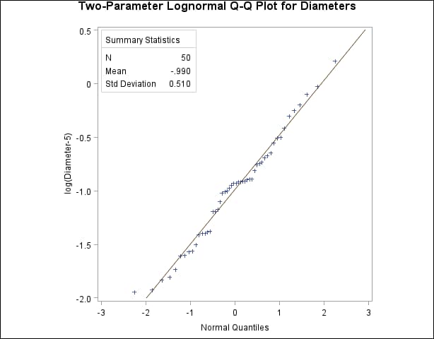
Because the point pattern in Output 4.33.1 is linear, you can estimate the lognormal parameters ![]() and
and ![]() as the normal plot estimates of
as the normal plot estimates of ![]() and
and ![]() , which are
, which are ![]() 0.99 and 0.51. These values correspond to the previous estimates of
0.99 and 0.51. These values correspond to the previous estimates of ![]() 0.92 for
0.92 for ![]() and 0.5 for
and 0.5 for ![]() from Example 4.31. A sample program for this example, uniex18.sas, is available in the SAS Sample Library for Base SAS software.
from Example 4.31. A sample program for this example, uniex18.sas, is available in the SAS Sample Library for Base SAS software.