The UNIVARIATE Procedure

Example 4.36 Creating a P-P Plot

The distances between two holes cut into 50 steel sheets are measured and saved as values of the variable Distance in the following data set:

data Sheets;
   input Distance @@;
   label Distance='Hole Distance in cm';
   datalines;
 9.80 10.20 10.27  9.70  9.76
10.11 10.24 10.20 10.24  9.63
 9.99  9.78 10.10 10.21 10.00
 9.96  9.79 10.08  9.79 10.06
10.10  9.95  9.84 10.11  9.93
10.56 10.47  9.42 10.44 10.16
10.11 10.36  9.94  9.77  9.36
 9.89  9.62 10.05  9.72  9.82
 9.99 10.16 10.58 10.70  9.54
10.31 10.07 10.33  9.98 10.15
;

It is decided to check whether the distances are normally distributed. The following statements create a P-P plot, shown in Output 4.36.1, which is based on the normal distribution with mean $\mu =10$ and standard deviation $\sigma =0.3$ :

title 'Normal Probability-Probability Plot for Hole Distance';
ods graphics on;
proc univariate data=Sheets noprint;
   ppplot Distance / normal(mu=10 sigma=0.3)
                     square;
run;

The NORMAL option in the PPPLOT statement requests a P-P plot based on the normal cumulative distribution function, and the MU= and SIGMA= normal-options specify $\mu$ and $\sigma$ . Note that a P-P plot is always based on a completely specified distribution—in other words, a distribution with specific parameters. In this example, if you did not specify the MU= and SIGMA= normal-options, the sample mean and sample standard deviation would be used for $\mu$ and $\sigma$ .

Output 4.36.1: Normal P-P Plot with Diagonal Reference Line

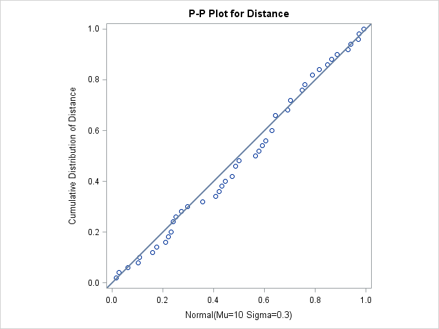
The linearity of the pattern in Output 4.36.1 is evidence that the measurements are normally distributed with mean 10 and standard deviation 0.3. The SQUARE option displays the plot in a square format.