The QLIM Procedure

This example illustrates how to use the QLIM procedure to perform Bayesian analysis. The generated data mimic a hypothetical scenario in which you study the number of tickets sold for a sports event given the probability of the hosting team winning and the price of the tickets. The following statements create the dataset:

title1 'Bayesian Analysis';

ods graphics on;

data test;
   do i=1 to 200;
      e1 = rannor(8726)*2000;
      WinChance = ranuni(8772);
      Price = 10+ranexp(8773)*4;
      y = 48000 + 5000*WinChance - 100 * price +  e1;
      if y>50000 then TicketSales = 50000;
      if y<=50000 then TicketSales = y;
      output;
   end;
   keep WinChance price  y TicketSales;
run;

The following statements perform Bayesian analysis of a Tobit model:

proc qlim data=test plots(prior)=all;
   model TicketSales = WinChance price;
   endogenous TicketSales ~ censored(lb=0 ub= 50000);
   prior intercept~normal(mean=48000);
   prior WinChance~normal(mean=5000);
   prior Price~normal(mean=-100);
   bayes NBI=10000 NMC=30000 THIN=1 ntrds=1 DIAG=ALL STATS=ALL seed=2;
run;

Output 29.8.1 shows the results from the maximum likelihood estimation and the Bayesian analysis with diffuse prior of this Tobit model.

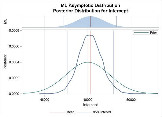
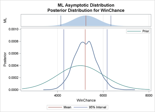
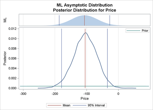
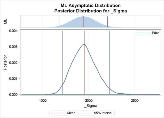
Output 29.8.2 depicts a graphical representation of MLE, prior, and posterior distributions.

Output 29.8.2: Predictive Analysis by Observation Number

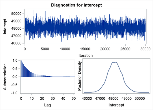
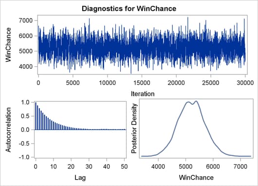
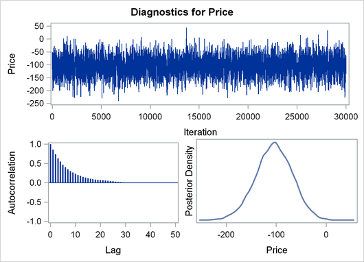
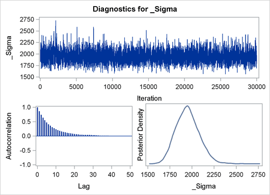
The validity of the MCMC sampling phase can be monitored with Output 29.8.3.

Output 29.8.3: Predictive Analysis by Observation Number

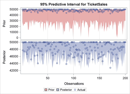
Finally the prior and the posterior predictive analyses are represented in Output 29.8.4

Output 29.8.4: Predictive Analysis by Observation Number