The QLIM Procedure
- Overview
-
Getting Started

-
Syntax
-
DetailsOrdinal Discrete Choice ModelingLimited Dependent Variable ModelsStochastic Frontier Production and Cost ModelsHeteroscedasticity and Box-Cox TransformationBivariate Limited Dependent Variable ModelingSelection ModelsMultivariate Limited Dependent ModelsVariable SelectionTests on ParametersEndogeneity and Instrumental VariablesPanel Data AnalysisBayesian AnalysisPrior DistributionsAutomated MCMCMarginal LikelihoodStandard DistributionsOutput to SAS Data SetOUTEST= Data SetNamingODS Table NamesODS Graphics
-
Examples
- References
Limited Dependent Variable Models
Censored Regression Models
When the dependent variable is censored, values in a certain range are all transformed to a single value. For example, the standard tobit model can be defined as
![\[ y^{*}_{i} = \mathbf{x}_{i}’\bbeta + \epsilon _{i} \]](images/etsug_qlim0051.png)
![\[ y_{i} = \left\{ \begin{array}{ll} y^{*}_{i} & \mr{if} y^{*}_{i}>0 \\ 0 & \mr{if} y^{*}_{i}\leq 0 \end{array} \right. \]](images/etsug_qlim0110.png)
where  . The log-likelihood function of the standard censored regression model is
![\[ \ell = \sum _{i\in \{ y_{i}=0\} }\ln [1-\Phi (\mathbf{x}_{i}’\bbeta /\sigma )] +\sum _{i\in \{ y_{i}>0\} } \ln \left[\phi (\frac{y_{i}-\mathbf{x}_{i}'\bbeta }{\sigma })/\sigma \right] \]](images/etsug_qlim0112.png)
where  is the cumulative density function of the standard normal distribution and
  is the probability density function of the standard normal distribution.
The tobit model can be generalized to handle observation-by-observation censoring. The censored model on both of the lower and upper limits can be defined as
![\[ y_{i} = \left\{ \begin{array}{ll} R_{i} & \mr{if} \; y_{i}^{*} \geq R_{i} \\ y_{i}^{*} & \mr{if} \; L_{i} < y_{i}^{*} < R_{i} \\ L_{i} & \mr{if} \; y_{i}^{*} \leq L_{i} \end{array} \right. \]](images/etsug_qlim0115.png)
The log-likelihood function can be written as
![\begin{eqnarray*} \ell & = & \sum _{i\in \{ L_{i}< y_{i} < R_{i}\} } \ln \left[\phi (\frac{y_{i}-\mathbf{x}_{i}'\bbeta }{\sigma })/\sigma \right] + \sum _{i\in \{ y_{i}=R_{i}\} } \ln \left[\Phi (-\frac{R_{i}-\mathbf{x}_{i}'\bbeta }{\sigma })\right] + \\ & & \sum _{i\in \{ y_{i}=L_{i}\} } \ln \left[\Phi (\frac{L_{i}-\mathbf{x}_{i}'\bbeta }{\sigma })\right] \end{eqnarray*}](images/etsug_qlim0116.png)
Log-likelihood functions of the lower- or upper-limit censored model are easily derived from the two-limit censored model. The log-likelihood function of the lower-limit censored model is
![\[ \ell = \sum _{i\in \{ y_{i} > L_{i}\} } \ln \left[\phi (\frac{y_{i}-\mathbf{x}_{i}'\bbeta }{\sigma })/\sigma \right] + \sum _{i\in \{ y_{i}=L_{i}\} } \ln \left[\Phi (\frac{L_{i}-\mathbf{x}_{i}'\bbeta }{\sigma })\right] \]](images/etsug_qlim0117.png)
The log-likelihood function of the upper-limit censored model is
![\[ \ell = \sum _{i\in \{ y_{i} < R_{i}\} } \ln \left[\phi (\frac{y_{i}-\mathbf{x}_{i}'\bbeta }{\sigma })/\sigma \right] + \sum _{i\in \{ y_{i}=R_{i}\} } \ln \left[1-\Phi (\frac{R_{i}- \mathbf{x}_{i}'\bbeta }{\sigma })\right] \]](images/etsug_qlim0118.png)
Types of Tobit Models
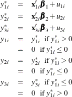
Amemiya (1984) classified Tobit models into five types based on characteristics of the likelihood function. For notational convenience,
let P denote a distribution or density function,  is assumed to be normally distributed with mean
  and variance
  .
.
Type 1 Tobit
The Type 1 Tobit model was already discussed in the preceding section.
The likelihood function is characterized as  .
.
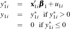
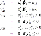
Type 2 Tobit
The Type 2 Tobit model is defined as
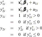
where  . The likelihood function is described as
  .
.
Type 3 Tobit
The Type 3 Tobit model is different from the Type 2 Tobit in that  of the Type 3 Tobit is observed when
  .
.
where 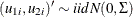 .
.
The likelihood function is characterized as 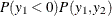 . Type 4 Tobit
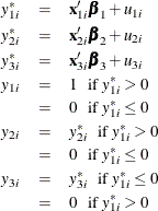
The Type 4 Tobit model consists of three equations:
where 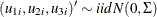 . The likelihood function of the Type 4 Tobit model is characterized as
 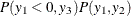 .
.
Type 5 Tobit
The Type 5 Tobit model is defined as follows:
where  are from iid trivariate normal distribution. The likelihood function of the Type 5 Tobit model is characterized as
 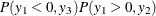 .
.
Code examples for these models can be found in Types of Tobit Models.
Truncated Regression Models
In a truncated model, the observed sample is a subset of the population where the dependent variable falls in a certain range.
For example, when neither a dependent variable nor exogenous variables are observed for  , the truncated regression model can be specified.
![\[ \ell = \sum _{i\in \{ y_{i}\geq 0\} } \left\{ -\ln \Phi (\mathbf{x}_{i}’\bbeta /\sigma ) + \ln \left[\frac{\phi ((y_{i} - \mathbf{x}_{i}'\bbeta )/\sigma )}{\sigma } \right] \right\} \]](images/etsug_qlim0139.png)
Two-limit truncation model is defined as
![\[ y_{i} = y_{i}^{*} \mr{if} \; L_{i} \leq y_{i}^{*} \leq R_{i} \]](images/etsug_qlim0140.png)
The log-likelihood function of the two-limit truncated regression model is
![\[ \ell = \sum _{i=1}^{N} \left\{ \ln \left[\phi (\frac{y_{i}-\mathbf{x}_{i}'\bbeta }{\sigma })/\sigma \right] - \ln \left[\Phi (\frac{R_{i}-\mb{x}_{i}'\bbeta }{\sigma }) - \Phi (\frac{L_{i}-\mb{x}_{i}'\bbeta }{\sigma })\right] \right\} \]](images/etsug_qlim0141.png)
The log-likelihood functions of the lower- and upper-limit truncation model are
![\begin{eqnarray*} \ell & = & \sum _{i=1}^{N}\left\{ \ln \left[\phi (\frac{y_{i}-\mb{x}_{i}'\bbeta }{\sigma }) / \sigma \right] - \ln \left[1 - \Phi (\frac{L_{i}-\mb{x}_{i}'\bbeta }{\sigma })\right] \right\} \; \; \textrm{(lower)} \\ \ell & = & \sum _{i=1}^{N}\left\{ \ln \left[\phi (\frac{y_{i}-\mb{x}_{i}'\bbeta }{\sigma }) / \sigma \right] - \ln \left[\Phi (\frac{R_{i}-\mb{x}_{i}'\bbeta }{\sigma })\right] \right\} \; \; \textrm{(upper)} \end{eqnarray*}](images/etsug_qlim0142.png)