The QLIM Procedure
- Overview
-
Getting Started

-
Syntax
-
DetailsOrdinal Discrete Choice ModelingLimited Dependent Variable ModelsStochastic Frontier Production and Cost ModelsHeteroscedasticity and Box-Cox TransformationBivariate Limited Dependent Variable ModelingSelection ModelsMultivariate Limited Dependent ModelsVariable SelectionTests on ParametersEndogeneity and Instrumental VariablesPanel Data AnalysisBayesian AnalysisPrior DistributionsAutomated MCMCMarginal LikelihoodStandard DistributionsOutput to SAS Data SetOUTEST= Data SetNamingODS Table NamesODS Graphics
-
Examples
- References
Bivariate Limited Dependent Variable Modeling
The generic form of a bivariate limited dependent variable model is
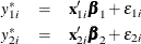
where the disturbances,  and
and  , have joint normal distribution with zero mean, standard deviations
  and
and  , and correlation of
  .
.  and
and  are latent variables. The dependent variables
  and
and  are observed if the latent variables and fall in certain ranges:
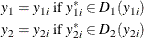
D is a transformation from  to
to  . For example, if
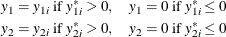
  and
and  are censored variables with lower bound 0, then
There are three cases for the log likelihood of . The first case is that  and
and  . That is, this observation is mapped to one point in the space of latent variables. The log likelihood is computed from a
bivariate normal density,
. That is, this observation is mapped to one point in the space of latent variables. The log likelihood is computed from a
bivariate normal density,
![\[ \ell _{i} = \ln \left[\phi _2(\frac{y_1-\mb{x_1}'\bbeta _1}{\sigma _1}, \frac{y_2-\mb{x_2}'\bbeta _2}{\sigma _2}, \rho )\right] - \ln \sigma _1 - \ln \sigma _2 \]](images/etsug_qlim0203.png)
where  is the density function for standardized bivariate normal distribution with correlation ,
![\[ \phi _2(u,v,\rho ) = \frac{e^{-(1/2)(u^2+v^2-2\rho uv)/(1-\rho ^2)}}{2\pi (1-\rho ^2)^{1/2}} \]](images/etsug_qlim0205.png)
The second case is that one observed dependent variable is mapped to a point of its latent variable and the other dependent
variable is mapped to a segment in the space of its latent variable. For example, in the bivariate censored model specified,
if observed  and
and  , then
  and
and ![$y2^*\in (-\infty , 0]$](images/etsug_qlim0209.png) . In general, the log likelihood for one observation can be written as follows (the subscript i is dropped for simplicity): If one set is a single point and the other set is a range, without loss of generality, let
. In general, the log likelihood for one observation can be written as follows (the subscript i is dropped for simplicity): If one set is a single point and the other set is a range, without loss of generality, let  and
and ![$D_2(y_2) = [L_2, R_2]$](images/etsug_qlim0211.png) ,
,
![\begin{eqnarray*} \ell _{i} & =& \ln \left[\phi (\frac{y_1-\mb{x_1}'\bbeta _1}{\sigma _1})\right] - \ln \sigma _1 \\ & +& \ln \left[\Phi \left(\frac{R_2-\mb{x_2}'\bbeta _2 -\rho \frac{y_1-\mb{x_1}'\bbeta _1}{\sigma _1}}{\sigma _2}\right) - \Phi \left(\frac{L_2-\mb{x_2}'\bbeta _2 -\rho \frac{y_1-\mb{x_1}'\bbeta _1}{\sigma _1}}{\sigma _2}\right)\right] \end{eqnarray*}](images/etsug_qlim0212.png)
where  and
and  are the density function and the cumulative probability function for standardized univariate normal distribution.
The third case is that both dependent variables are mapped to segments in the space of latent variables. For example, in the
bivariate censored model specified, if observed  and , then
 ![$y1^* \in (-\infty , 0]$](images/etsug_qlim0216.png) and . In general, if
and . In general, if ![$D_1(y_1) = [L_1, R_1]$](images/etsug_qlim0217.png) and , the log likelihood is
and , the log likelihood is
![\[ \ell _{i} = \ln \int _{\frac{L_1-\mb{x_1}'\bbeta _1}{\sigma _1}} ^{\frac{R_1-\mb{x_1}'\bbeta _1}{\sigma _1}} \int _{\frac{L_2-\mb{x_2}'\bbeta _2}{\sigma _2}} ^{\frac{R_2-\mb{x_2}'\bbeta _2}{\sigma _2}} \phi _2(u,v,\rho ) \, du\, dv \]](images/etsug_qlim0218.png)