The QLIM Procedure
- Overview
-
Getting Started

-
Syntax
-
DetailsOrdinal Discrete Choice ModelingLimited Dependent Variable ModelsStochastic Frontier Production and Cost ModelsHeteroscedasticity and Box-Cox TransformationBivariate Limited Dependent Variable ModelingSelection ModelsMultivariate Limited Dependent ModelsVariable SelectionTests on ParametersEndogeneity and Instrumental VariablesPanel Data AnalysisBayesian AnalysisPrior DistributionsAutomated MCMCMarginal LikelihoodStandard DistributionsOutput to SAS Data SetOUTEST= Data SetNamingODS Table NamesODS Graphics
-
Examples
- References
Panel Data Analysis
You can use panel data to estimate the random effects in linear, censored response, truncated response, discrete choice, and stochastic frontier models.
Random-Effects Models for Panel Data
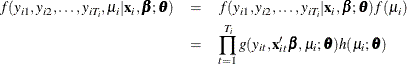
The general form of a nonlinear random-effects model is defined by the density for an observed random variable,  , as follows[13]
![\[ f(y_{it}|\mathbf{x}_{it}, \mu _ i) = g(y_{it}, \mathbf{x}_{it}’\bbeta , \mu _ i; \btheta ) \]](images/etsug_qlim0332.png)
where  is a vector of ancillary parameters such as a scale parameter or an overdispersion parameter and
  ,
,  , embodies the group-specific heterogeneity, which is unobservable and has the density
![\[ f(\mu _ i) = h(\mu _ i ; \btheta ) \]](images/etsug_qlim0336.png)
There are  observations for group i. For example, in the case of a random-effects Tobit model, is specified as
![\[ y^{*}_{it} = \mathbf{x}_{it}’\bbeta + \epsilon _{it}, ~ ~ ~ ~ ~ ~ ~ t=1,\ldots ,T_ i, ~ ~ ~ i=1,\ldots ,N \]](images/etsug_qlim0338.png)
![\[ y_{it} = \left\{ \begin{array}{ll} y^{*}_{it} & \mr{if} y^{*}_{it}>0 \\ 0 & \mr{if} y^{*}_{it}\leq 0 \end{array} \right. \]](images/etsug_qlim0339.png)
where
![\[ \epsilon _{it} = \mu _{i} + v_{it} \]](images/etsug_qlim0340.png)
![\[ v_{it}|\mathbf{x}_{i}, \mu _ i \sim N(0,\sigma ^{2}) \]](images/etsug_qlim0341.png)
![\[ \mu _{i}|\mathbf{x}_{i} \sim N(0,\sigma ^{2}_{\mu }) \]](images/etsug_qlim0342.png)
where  contains
  for all t and consists of
  and
and  . Therefore, for this model
![\[ f(y_{it}|\mathbf{x}_{it}, \mu _ i) = \{ 1 - \Phi [(\mathbf{x}_{it}’\bbeta + \mu _{i})/\sigma ]\} ^{1[y_{it}=0]}\{ (1/\sigma )\phi [(y_{it} - \mathbf{x}_{it}’\bbeta - \mu _{i})/\sigma ]\} ^{1[y_{it}>0]} \]](images/etsug_qlim0346.png)
and
![\[ f(\mu _ i) = \phi (\mu _ i/\sigma _{\mu }) \]](images/etsug_qlim0347.png)
where  is the cumulative density function and
  is the probability density function of the standard normal distribution and
 ![$1[\cdot ]$](images/etsug_qlim0348.png) is the indicator function.
is the indicator function.
By construction, the observations in group i are correlated and jointly distributed with a distribution that does not factor into the product of the marginal distributions.
To be able to drive the joint distribution of the  random variables,
  , the assumption that the observations are independent conditional on is important. Under this assumption the joint distribution can be written as
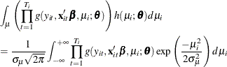
In order to form the likelihood function for the observed data, the unobserved component, , must be integrated out. For individual i
![\[ L_ i = f(y_{i1}, y_{i2},\ldots , y_{iT_ i} | \mathbf{x}_{i}, \bbeta ; \btheta ) = \int _{\mu } \left[\prod _{t=1}^{T_ i} g(y_{it}, \mathbf{x}_{it}’\bbeta , \mu _ i; \btheta )\right] h(\mu _ i ; \btheta )d\mu _ i \]](images/etsug_qlim0352.png)
Therefore, the log-likelihood function for the observed data becomes
![\[ \ln L = \sum _{i=1}^ N \ln \left[ \int _{\mu } \left(\prod _{t=1}^{T_ i} g(y_{it}, \mathbf{x}_{it}’\bbeta , \mu _ i; \btheta )\right)h(\mu _ i ; \btheta )d\mu _ i\right] \]](images/etsug_qlim0353.png)
In most cases, the integral in the square brackets does not have a closed form. The following subsections describe three approaches to this integration.
Simulated Maximum Likelihood
You can use simulation to approximate the integral. First, note that
![\[ \int _{\mu } \left(\prod _{t=1}^{T_ i} g(y_{it}, \mathbf{x}_{it}’\bbeta , \mu _ i; \btheta )\right)h(\mu _ i ; \btheta )d\mu _ i = E[F(\mu _ i;\btheta )] \]](images/etsug_qlim0354.png)
The function is smooth, continuous, and continuously differentiable. By the law of large numbers, if 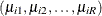 is a sample of iid draws from
  , then
![\[ \mr{plim}\frac{1}{R}\sum _{r=1}^{R} F(\mu _{ir};\btheta ) = E[F(\mu _ i;\btheta )] \]](images/etsug_qlim0357.png)
This operation is implemented by simulation that uses a random-number generator. PROC QLIM inserts the simulated integral in the log likelihood to obtain the simulated log likelihood
![\[ \ln L_{Simulated} = \sum _{i=1}^ N \ln \left[ \frac{1}{R}\sum _{r=1}^{R} \left(\prod _{t=1}^{T_ i} g(y_{it}, \mathbf{x}_{it}’\bbeta , \mu _{ir}; \btheta )\right)\right] \]](images/etsug_qlim0358.png)
and maximizes the simulated log likelihood with respect to the parameters  and .
and .
Under certain assumptions (Greene 2001), the simulated likelihood estimator and the maximum likelihood estimator are equivalent. For this equivalence result to
hold, the number of draws, R, must increase faster than the number of observations, N. For this reason, if the NDRAW option is not specified, then by default, it is tied to the sample size by using the rule
 , where
  .
.
The use of independent random draws in simulation is conceptually straightforward, and the statistical properties of the simulated maximum likelihood estimator are easy to derive. However, simulation is a very computationally intensive technique. Moreover, the simulation method itself contributes to the variation of the simulated maximum likelihood estimator; see, for example, Geweke (1995). There are other ways to take draws that can provide greater accuracy by covering the domain of the integral more uniformly and by lowering the simulation variance (Train 2009 section 9.3). Quas–Monte Carlo methods (QMC), for example, are based on an integration technique that replaces the pseudorandom draws of Monte Carlo (MC) integration with a sequence of judiciously selected nonrandom points that provide more uniform coverage of the domain of the integral. Therefore, the advantage of QMC integration over MC integration is that for some types of sequences, the accuracy is far greater, convergence is much faster, and the simulation variance is smaller. QMC methods are surveyed in Bhat (2001), Sloan and Woźniakowski (1998), and Morokoff and Caflisch (1995). Besides MC simulation, PROC QLIM offers the QMC integration method that uses Halton sequences.
QMC Method Using the Halton Sequence
Halton sequences (Halton 1960) provide a uniform coverage for each observations’s integral, and they decrease the simulation variance by inducing a negative correlation over the draws for each observation. A Halton sequence is constructed deterministically in terms of a prime number as its base. For example, the following sequence is the Halton sequence for 2:
![\[ 1/2, 1/4, 3/4, 1/8, 5/8, 3/8, 7/8, 1/16, 9/16, \ldots \]](images/etsug_qlim0361.png)
For more information about how to generate a Halton sequence, see Train (2009) section 9.3.3.
If you use the QMC method, one long Halton sequence is created, and then part of the sequence (or the whole sequence, depending on whether you decide to discard the initial elements of the sequence[14]) is used in groups. Each group of consequent elements constitutes the “draws” for each cross-sectional observation. This way, each subsequence fills in the gaps for the previous subsequences, and the draws for one observation tend to be negatively correlated with those for the previous observation.
When the number of draws used for each observation rises, the coverage for each observation improves. This improvement in turn improves the accuracy; however, the negative covariance across observations diminishes. Because Halton draws are far more effective than random draws for simulation, a small number of Halton draws provide relatively good integration (Spanier and Maize 1991).
The Halton draws are for a uniform density. PROC QLIM evaluates the inverse cumulative standard normal density for each element of the Halton sequence to obtain draws from a standard normal density.
Approximation by Hermite Quadrature
This method is the Butler and Moffitt (1982) approach, which is based on models in which has a normal distribution. If is normally distributed with zero mean, then
Let  . Then
  and
and 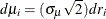 . Making the change of variable and letting the error effects be additive produce
![\[ L_ i = \frac{1}{\sqrt {\pi }} \int _{-\infty }^{+\infty } \exp (-r_ i^2) \left[\prod _{t=1}^{T_ i} g(y_{it}, \mathbf{x}_{it}’\bbeta + (\sigma _{\mu }\sqrt {2})r_ i; \btheta )\right] dr_ i \]](images/etsug_qlim0366.png)
This likelihood function is in a form that can be approximated accurately by using Gauss-Hermite quadrature, which eliminates the integration. Thus, the log-likelihood function can be approximated with
![\[ \ln L_{h} = \sum _{i=1}^ N \ln \left[ \frac{1}{\sqrt {\pi }}\sum _{h=1}^{H} w_ h \prod _{t=1}^{T_ i} g(y_{it}, \mathbf{x}_{it}’\bbeta + (\sigma _{\mu }\sqrt {2})r_ i; \btheta )\right] \]](images/etsug_qlim0367.png)
where  and
and  are the weights and nodes for the Hermite quadrature of degree H. PROC QLIM maximizes
  when the Hermite quadrature option is specified (METHOD=HERMITE in the RANDOM statement).
[13] The i subscript represents individuals, and the t subscript represents time.
[14] When sequences are created in multiple dimensions, the initial part of the series is usually eliminated because the initial terms of multiple Halton sequences are highly correlated. However, there is no such correlation for a single dimension.