The QLIM Procedure

BAYES Statement

BAYES <options>;

The BAYES statement controls the Metropolis sampling scheme that is used to obtain samples from the posterior distribution of the underlying model and data.

AGGREGATION=WEIGHTED |NOWEIGHTED

specifies how multiple posterior samples should be aggregated. AGGREGATION=WEIGHTED implements a weighted resampling scheme for the aggregation of multiple posterior chains. You can use this option when the posterior distribution is characterized by several very distinct posterior modes. AGGREGATION=NOWEIGHTED aggregates multiple posterior chains without any adjustment. You can use this option when the posterior distribution is characterized by one or few relatively close posterior modes. By default, AGGREGATION=NOWEIGHTED. For more information, see the section Aggregation of Multiple Chains.

AUTOMCMC <=(automcmc-options)>

specifies an algorithm for the auto-initialization of the MCMC sampling algorithm. For more information, see the section Automated Initialization of MCMC.

ACCURACY= (accuracy-options)

customizes the behavior of the AUTOMCMC algorithm when you are searching for an accurate representation of the posterior distribution. You can specify the following accuracy-options:

ATTEMPTS=number

specifies the maximum number of attempts that is required in order to obtain accurate samples from the posterior distribution. By default,ATTEMPTS=10.

TARGETESS=number

requests that the accuracy search be based on the effective sample size (ESS) analysis. If you specify this option, you must also specify the minimum number of effective samples.

TARGETSTATS<=(targetstats-option)>

requests that the accuracy search be based on the analysis of the posterior mean and a posterior quantile of interest. You can customize the behavior of the analysis of the posterior mean by adjusting HEIDELBERGER sub-options. You can customize the behavior of the analysis of the posterior quantile by adjusting the RAFTERY sub-options. If you specify TARGETSTATS,, you can also specify how the Raftery-Lewis test should be interpreted by using the following option:

RLLIMITS=(LB=number UB=number): specifies a region where the search for the optimal sample size depends directly on the Raftery-Lewis test. By default, RLLIMITS (LB=10000 UB=300000).

TOL=value

specifies the proportion of parameters that are required to be accurate. By default, TOL=0.95.

MAXNMC=number

specifies the maximum number of posterior samples that the AUTOMCMC option allows. By default, MAXNMC=700000.

RANDINIT <=(randinit-options)>

specifies random starting points for the MCMC algorithm. The starting points can be sampled around the maximum likelihood estimate and around the prior mean. You can specify the following randinit-options:

MULTIPLIER= (value): specifies the radius of the area where the starting points are sampled. For the starting points that are sampled around the maximum likelihood estimate, the radius equals the standard deviation of the maximum likelihood estimate multiplied by the multiplier value. For the starting points that are sampled around the prior mean, the radius equals the standard deviation of the prior distribution multiplied by the multiplier value. By default, MULTIPLIER=2.
PROPORTION= (value): specifies the proportion of starting points that are sampled around the maximum likelihood estimate and around the prior mean. By default, PROPORTION=0, which implies that all the initial points are sampled around the maximum likelihood estimate. If you use choose to sample starting points around the prior mean, the convergence of the MCMC algorithm could be very slow.

STATIONARITY= (stationarity-options)

customizes the behavior of the AUTOMCMC algorithm when you are trying to sample from the posterior distribution. You can specify the following accuracy-options:

ATTEMPTS=number: specifies the maximum number of attempts that are required in order to obtain stationary samples from the posterior distribution. By default, ATTEMPTS=10.
TOL=value: specifies the proportion of parameter whose samples must to be stationary. By default, TOL=0.95.

DIAGNOSTICS=ALL | NONE | (keyword-list) DIAG=ALL | NONE | (keyword-list)

controls which diagnostics are produced. All the following diagnostics are produced with DIAGNOSTICS=ALL. If you do not want any of these diagnostics, specify DIAGNOSTICS=NONE. If you want some but not all of the diagnostics, or if you want to change certain settings of these diagnostics, specify a subset of the following keywords. By default, DIAGNOSTICS=NONE.

AUTOCORR <(LAGS= numeric-list)>

computes the autocorrelations at lags that are specified in the numeric-list. Elements in the numeric-list are truncated to integers, and repeated values are removed. If the LAGS= option is not specified, autocorrelations of lags 1, 5, 10, and are computed.

ESS

computes Carlin’s estimate of the effective sample size, the correlation time, and the efficiency of the chain for each parameter.

GEWEKE <(geweke-options)>

computes the Geweke spectral density diagnostics, which are essentially a two-sample t test between the first $f_1$ portion and the last $f_2$ portion of the chain. The default is $f_1=0.1$ and $f_2=0.5$ , but you can choose other fractions by using the following geweke-options:

FRAC1=value: specifies the fraction $f_1$ for the first window.
FRAC2=value: specifies the fraction $f_2$ for the second window.

HEIDELBERGER <(heidel-options)>

computes the Heidelberger and Welch diagnostic for each variable, which consists of a stationarity test of the null hypothesis that the sample values form a stationary process. If the stationarity test is not rejected, a halfwidth test is then carried out. Optionally, you can specify one or more of the following heidel-options:

SALPHA=value: specifies the $\alpha$ level $(0<\alpha <1)$ for the stationarity test.
HALPHA=value: specifies the $\alpha$ level $(0<\alpha <1)$ for the halfwidth test.
EPS=value: specifies a positive number $\epsilon$ such that if the halfwidth is less than $\epsilon$ times the sample mean of the retained iterates, the halfwidth test is passed.

MCSE MCERROR

computes the Monte Carlo standard error for each parameter. The Monte Carlo standard error, which measures the simulation accuracy, is the standard error of the posterior mean estimate and is calculated as the posterior standard deviation divided by the square root of the effective sample size.

RAFTERY<(raftery-options)>

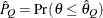computes the Raftery and Lewis diagnostics, which evaluate the accuracy of the estimated quantile ( $\hat{\theta }_ Q$ for a given $Q \in (0,1)$ ) of a chain. $\hat{\theta }_ Q$ can achieve any degree of accuracy when the chain is allowed to run for a long time. The computation is stopped when the estimated probability $\hat{P}_ Q= \mr{Pr}(\theta \leq \hat{\theta }_ Q)$ reaches within $\pm R$ of the value $Q$ with probability $S$ ; that is, $\mr{Pr}(Q-R \leq \hat{P}_ Q \leq Q+R)=S$ . The following raftery-options enable you to specify $Q, R, S$ , and a precision level $\epsilon$ for the test:

QUANTILE | Q=value: specifies the order (a value between 0 and 1) of the quantile of interest. The default is 0.025.
ACCURACY | R=value: specifies a small positive number as the margin of error for measuring the accuracy of estimation of the quantile. The default is 0.005.
PROBABILITY | S=value: specifies the probability of attaining the accuracy of the estimation of the quantile. The default is 0.95.
EPSILON | EPS=value: specifies the tolerance level (a small positive number) for the stationary test. The default is 0.001.

MINTUNE=number

specifies the minimum number of tuning phases. The default is 2.

MAXTUNE=number

specifies the maximum number of tuning phases. The default is 24.

NBI=number

specifies the number of burn-in iterations before the chains are saved. The default is 1,000.

NMC=number

specifies the number of iterations after the burn-in. The default is 1,000.

NMCPRIOR=number

specifies the number of samples for the prior predictive analysis when PLOTS(PRIOR)=BAYESPRED is requested. The default is 10,000.

NTRDS=number THREADS=number

specifies the number of threads to be used. The number of threads cannot exceed the number of computer cores available. Each core samples the number of iterations that is specified by the NMC option. The default is 1.

NTU=number

specifies the number of samples for each tuning phase. The default is 500.

OUTPOST=SAS-data-set

names the SAS data set to contain the posterior samples. Alternatively, you can create the output data set by specifying an ODS OUTPUT statement as follows:

ODS OUTPUT POSTERIORSAMPLE = <SAS-data-set>;

OUTPRIOR=SAS-data-set

names the SAS data set to contain the prior samples used to generate the prior predictive analysis when you request the prior predictive plots. Alternatively, you can create the output data set by specifying an ODS OUTPUT statement as follows:

ODS OUTPUT PRIORSAMPLE = <SAS-data-set>;

PROPCOV=value

specifies the method used in constructing the initial covariance matrix for the Metropolis-Hastings algorithm. The QUANEW and NMSIMP methods find numerically approximated covariance matrices at the optimum of the posterior density function with respect to all continuous parameters. The tuning phase starts at the optimized values; in some problems, this can greatly increase convergence performance. If the approximated covariance matrix is not positive definite, then an identity matrix is used instead. You can specify the following values:

CONGRA: performs a conjugate-gradient optimization.
DBLDOG: performs a version of double-dogleg optimization.
NEWRAP: performs a Newton-Raphson optimization that combines a line-search algorithm with ridging.
NMSIMP: performs a Nelder-Mead simplex optimization.
NRRIDG: performs a Newton-Raphson optimization with ridging.
QUANEW: performs a quasi-Newton optimization.
TRUREG: performs a trust-region optimization.

SAMPLING=MULTIMETROPOLIS |UNIMETROPOLIS |MODELMETROPOLIS

specifies how to sample from the posterior distribution. SAMPLING=MULTIMETROPOLIS implements a Metropolis sampling scheme on a single block that contains all the parameters of the model. SAMPLING=MODELMETROPOLIS implements a Metropolis sampling scheme on multiple blocks: one block for each model (all the parameters of the model) plus a block for all the correlation parameters across the models. SAMPLING=UNIMETROPOLIS implements a Metropolis sampling scheme on multiple blocks, one for each parameter of the model. By default, SAMPLING=MULTIMETROPOLIS.

SEED=number

specifies an integer seed in the range 1 to $2^{31}-1$ for the random number generator in the simulation. Specifying a seed enables you to reproduce identical Markov chains for the same specification. If you do not specify the SEED= option, or if you specify a nonpositive seed, a random seed is derived from the time of day.

SIMTIME

prints the time required for the MCMC sampling.

controls the number of posterior statistics produced. Specifying STATISTICS=ALL is equivalent to specifying STATISTICS= (CORR COV INTERVAL PRIOR SUMMARY). If you do not want any posterior statistics, specify STATISTICS=NONE. The default is STATISTICS=(SUMMARY INTERVAL). You can specify the following global-options:

ALPHA=numeric-list: controls the probabilities of the credible intervals. The ALPHA= values must be between 0 and 1. Each ALPHA= value produces a pair of 100(1–ALPHA)% equal-tail and HPD intervals for each parameter. The default is ALPHA=0.05, which yields the 95% credible intervals for each parameter.
PERCENT=numeric-list: requests the percentile points of the posterior samples. The PERCENT= values must be between 0 and 100. The default is PERCENT=25, 50, 75, which yields the 25th, 50th, and 75th percentile points, respectively, for each parameter.

You can specify the following keywords:

CORR: produces the posterior correlation matrix.
COV: produces the posterior covariance matrix.
INTERVAL: produces equal-tail credible intervals and HPD intervals. The default is to produce the 95% equal-tail credible intervals and 95% HPD intervals, but you can use the ALPHA= global-option to request intervals of any probabilities.
NONE: suppresses printing of all summary statistics.
PRIOR: produces a summary table of the prior distributions used in the Bayesian analysis.
SUMMARY: produces the means, standard deviations, and percentile points (25th, 50th, and 75th) for the posterior samples. You can use the global PERCENT= global-option to request specific percentile points.

THIN=number THINNING=number

controls the thinning of the Markov chain. Only one in every k samples is used when THIN=k, and if NBI= $n_0$ and NMC=n, the number of samples that are kept is

$\biggl [ \frac{n_0+n}{k} \biggr ] - \biggl [ \frac{n_0}{k} \biggr ]$

where [a] represents the integer part of the number a. The default is THIN=1.