The QLIM Procedure
- Overview
-
Getting Started

-
Syntax
-
DetailsOrdinal Discrete Choice ModelingLimited Dependent Variable ModelsStochastic Frontier Production and Cost ModelsHeteroscedasticity and Box-Cox TransformationBivariate Limited Dependent Variable ModelingSelection ModelsMultivariate Limited Dependent ModelsVariable SelectionTests on ParametersEndogeneity and Instrumental VariablesBayesian AnalysisPrior DistributionsAutomated MCMCOutput to SAS Data SetOUTEST= Data SetNamingODS Table NamesODS Graphics
-
Examples
- References
Stochastic frontier production models were first developed by Aigner, Lovell, and Schmidt (1977); Meeusen and van den Broeck (1977). Specification of these models allow for random shocks of the production or cost but also include a term for technological or cost inefficiency. Assuming that the production function takes a log-linear Cobb-Douglas form, the stochastic frontier production model can be written as
where ![]() . The
. The ![]() term represents the stochastic error component and
term represents the stochastic error component and ![]() is the nonnegative, technology inefficiency error component. The
is the nonnegative, technology inefficiency error component. The ![]() error component is assumed to be distributed iid normal and independently from
error component is assumed to be distributed iid normal and independently from ![]() . If
. If ![]() , the error term,
, the error term, ![]() , is negatively skewed and represents technology inefficiency. If
, is negatively skewed and represents technology inefficiency. If ![]() , the error term
, the error term ![]() is positively skewed and represents cost inefficiency. PROC QLIM models the
is positively skewed and represents cost inefficiency. PROC QLIM models the ![]() error component as a half normal, exponential, or truncated normal distribution.
error component as a half normal, exponential, or truncated normal distribution.
In case of the normal-half normal model, ![]() is iid
is iid ![]() ,
, ![]() is iid
is iid ![]() with
with ![]() and
and ![]() independent of each other. Given the independence of error terms, the joint density of v and u can be written as
independent of each other. Given the independence of error terms, the joint density of v and u can be written as
Substituting ![]() into the preceding equation gives
into the preceding equation gives
Integrating u out to obtain the marginal density function of ![]() results in the following form:
results in the following form:
![\begin{eqnarray*} f(\epsilon ) & = & \int ^\infty _0 f(u,\epsilon )du \\ & = & \frac{2}{\sqrt {2\pi }\sigma } \left[ 1-\Phi \left( \frac{\epsilon \lambda }{\sigma } \right) \right] \exp \left\{ -\frac{\epsilon ^2}{2\sigma ^2} \right\} \\ & = & \frac{2}{\sigma }\phi \left( \frac{\epsilon }{\sigma } \right) \Phi \left( -\frac{\epsilon \lambda }{\sigma } \right) \end{eqnarray*}](images/etsug_qlim0162.png)
where ![]() and
and ![]() .
.
In the case of a stochastic frontier cost model, ![]() and
and
The log-likelihood function for the production model with ![]() producers is written as
producers is written as
Under the normal-exponential model, ![]() is iid
is iid ![]() and
and ![]() is iid exponential with scale parameter
is iid exponential with scale parameter ![]() . Given the independence of error term components
. Given the independence of error term components ![]() and
and ![]() , the joint density of v and u can be written as
, the joint density of v and u can be written as
The marginal density function of ![]() for the production function is
for the production function is
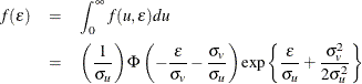
and the marginal density function for the cost function is equal to
The log-likelihood function for the normal-exponential production model with ![]() producers is
producers is
The normal-truncated normal model is a generalization of the normal-half normal model by allowing the mean of ![]() to differ from zero. Under the normal-truncated normal model, the error term component
to differ from zero. Under the normal-truncated normal model, the error term component ![]() is iid
is iid ![]() and
and ![]() is iid
is iid ![]() . The joint density of
. The joint density of ![]() and
and ![]() can be written as
can be written as
The marginal density function of ![]() for the production function is
for the production function is
![\begin{eqnarray*} f(\epsilon ) & = & \int ^\infty _0 f(u,\epsilon )du \\ & = & \frac{1}{ \sqrt {2\pi }\sigma \Phi \left( \mu /\sigma _ u \right) } \Phi \left( \frac{\mu }{\sigma \lambda }-\frac{\epsilon \lambda }{\sigma } \right) \exp \left\{ -\frac{(\epsilon +\mu )^2}{2\sigma ^2} \right\} \\ & = & \frac{1}{\sigma }\phi \left( \frac{\epsilon +\mu }{\sigma } \right) \Phi \left( \frac{\mu }{\sigma \lambda }-\frac{\epsilon \lambda }{\sigma } \right) \left[ \Phi \left( \frac{\mu }{\sigma _ u} \right) \right]^{-1} \end{eqnarray*}](images/etsug_qlim0175.png)
and the marginal density function for the cost function is
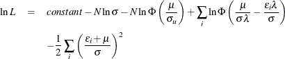
The log-likelihood function for the normal-truncated normal production model with ![]() producers is
producers is
For more detail on normal-half normal, normal-exponential, and normal-truncated models, see Kumbhakar and Lovell (2000); Coelli, Prasada Rao, and Battese (1998).