The QLIM Procedure
- Overview
-
Getting Started

-
Syntax
-
DetailsOrdinal Discrete Choice ModelingLimited Dependent Variable ModelsStochastic Frontier Production and Cost ModelsHeteroscedasticity and Box-Cox TransformationBivariate Limited Dependent Variable ModelingSelection ModelsMultivariate Limited Dependent ModelsVariable SelectionTests on ParametersEndogeneity and Instrumental VariablesBayesian AnalysisPrior DistributionsAutomated MCMCOutput to SAS Data SetOUTEST= Data SetNamingODS Table NamesODS Graphics
-
Examples
- References
To perform Bayesian analysis, you must specify a BAYES statement. Unless otherwise stated, all options in this section are options in the BAYES statement.
By default, PROC QLIM uses the random walk Metropolis algorithm to obtain posterior samples. For the implementation details of the Metropolis algorithm in PROC QLIM, such as the blocking of the parameters and tuning of the covariance matrices, see the sections Blocking of Parameters and Tuning the Proposal Distribution.
The Bayes theorem states that
where ![]() is a parameter or a vector of parameters and
is a parameter or a vector of parameters and ![]() is the product of the prior densities that are specified in the PRIOR
statement. The term
is the product of the prior densities that are specified in the PRIOR
statement. The term ![]() is the likelihood associated with the MODEL
statement.
is the likelihood associated with the MODEL
statement.
In a multivariate parameter model, all the parameters are updated in one single block (by default or when you specify the SAMPLING=MULTIMETROPOLIS option). This could be inefficient, especially when parameters have vastly different scales. As an alternative, you could update the parameters one at the time (by specifying SAMPLING=UNIMETROPOLIS).
One key factor in achieving high efficiency of a Metropolis-based Markov chain is finding a good proposal distribution for each block of parameters. This process is called tuning. The tuning phase consists of a number of loops controlled by the options MINTUNE and MAXTUNE. The MINTUNE= option controls the minimum number of tuning loops and has a default value of 2. The MAXTUNE= option controls the maximum number of tuning loops and has a default value of 24. Each loop is iterated the number of times specified by the NTU= option, which has a default of 500. At the end of every loop, PROC QLIM examines the acceptance probability for each block. The acceptance probability is the percentage of NTU proposed values that have been accepted. If this probability does not fall within the acceptance tolerance range (see the following section), the proposal distribution is modified before the next tuning loop.
A good proposal distribution should resemble the actual posterior distribution of the parameters. Large sample theory states that the posterior distribution of the parameters approaches a multivariate normal distribution (see Gelman et al. 2004, Appendix B; Schervish 1995, Section 7.4). That is why a normal proposal distribution often works well in practice. The default proposal distribution in PROC QLIM is the normal distribution.
The acceptance rate is closely related to the sampling efficiency of a Metropolis chain. For a random walk Metropolis, a
high acceptance rate means that most new samples occur right around the current data point. Their frequent acceptance means
that the Markov chain is moving rather slowly and not exploring the parameter space fully. A low acceptance rate means that
the proposed samples are often rejected; hence the chain is not moving much. An efficient Metropolis sampler has an acceptance
rate that is neither too high nor too low. The scale c in the proposal distribution ![]() effectively controls this acceptance probability. Roberts, Gelman, and Gilks (1997) show that if both the target and proposal densities are normal, the optimal acceptance probability for the Markov chain
should be around 0.45 in a one-dimension problem and should asymptotically approach 0.234 in higher-dimension problems. The
corresponding optimal scale is 2.38, which is the initial scale that is set for each block.
effectively controls this acceptance probability. Roberts, Gelman, and Gilks (1997) show that if both the target and proposal densities are normal, the optimal acceptance probability for the Markov chain
should be around 0.45 in a one-dimension problem and should asymptotically approach 0.234 in higher-dimension problems. The
corresponding optimal scale is 2.38, which is the initial scale that is set for each block.
Because of the nature of stochastic simulations, it is impossible to fine-tune a set of variables so that the Metropolis chain
has exactly the desired acceptance rate that you want. In addition, Roberts and Rosenthal (2001) empirically demonstrate that an acceptance rate between 0.15 and 0.5 is at least 80% efficient, so there is really no need
to fine-tune the algorithms to reach an acceptance probability that is within a small tolerance of the optimal values. PROC
QLIM works with a probability range, determined by ![]() . If the observed acceptance rate in a given tuning loop is less than the lower bound of the range, the scale is reduced;
if the observed acceptance rate is greater than the upper bound of the range, the scale is increased. During the tuning phase,
a scale parameter in the normal distribution is adjusted as a function of the observed acceptance rate and the target acceptance
rate. PROC QLIM uses the following updating scheme: [13]
. If the observed acceptance rate in a given tuning loop is less than the lower bound of the range, the scale is reduced;
if the observed acceptance rate is greater than the upper bound of the range, the scale is increased. During the tuning phase,
a scale parameter in the normal distribution is adjusted as a function of the observed acceptance rate and the target acceptance
rate. PROC QLIM uses the following updating scheme: [13]
where ![]() is the current scale,
is the current scale, ![]() is the current acceptance rate, and
is the current acceptance rate, and ![]() is the optimal acceptance probability.
is the optimal acceptance probability.
To tune a covariance matrix, PROC QLIM takes a weighted average of the old proposal covariance matrix and the recent observed covariance matrix, based on the number samples (as specified by the NTU= option) NTU samples in the current loop. The formula to update the covariance matrix is:
There are two ways to initialize the covariance matrix:
-
The default is an identity matrix that is multiplied by the initial scale of 2.38 and divided by the square root of the number of estimated parameters in the model. A number of tuning phases might be required before the proposal distribution is tuned to its optimal stage, because the Markov chain needs to spend time to learn about the posterior covariance structure. If the posterior variances of your parameters vary by more than a few orders of magnitude, if the variances of your parameters are much different from 1, or if the posterior correlations are high, then the proposal tuning algorithm might have difficulty forming an acceptable proposal distribution.
-
Alternatively, you can use a numerical optimization routine, such as the quasi-Newton method, to find a starting covariance matrix. The optimization is performed on the joint posterior distribution, and the covariance matrix is a quadratic approximation at the posterior mode. In some cases this is a better and more efficient way of initializing the covariance matrix. However, there are cases, such as when the number of parameters is large, where the optimization could fail to find a matrix that is positive definite. In those cases, the tuning covariance matrix is reset to the identity matrix.
A by-product of the optimization routine is that it also finds the maximum a posteriori (MAP) estimates with respect to the posterior distribution. The MAP estimates are used as the initial values of the Markov chain.
For more information, see the section INIT Statement.
You can assign initial values to any parameters. (For more information, see the INIT statement.) If you use the optimization option PROPCOV= , then PROC QLIM starts the tuning at the optimized values. This option overwrites the provided initial values. If you specify the RANDINIT option, the information that the INIT statement provides is overwritten.
When you want to exploit the possibility of running several MCMC instances at the same time (NTRDS=n>1), you face the problem of aggregating the chains. In ordinary applications, each MCMC instance can easily obtain stationary
samples from the entire posterior distribution. In these applications, you can use the option AGGREGATION=NOWEIGHTED. This
option piles up one chain on top of another and makes no particular adjustment. However, when the posterior distribution is
characterized by multiple distinct posterior modes, some of the MCMC instances fail to obtain stationary samples from the
entire posterior distribution. You can use the option AGGREGATION=WEIGHTED when the posterior samples from each MCMC instance
approximate well only a part of the posterior distribution.
The main idea behind the option AGGREGATION=WEIGHTED is to consider the entire posterior distribution to be similar to a mixture distribution. When you are sampling with multiple threads, each MCMC instance samples from one of the mixture components. Then the samples from each mixture component are aggregated together using a resampling scheme in which weights are proportional to the nonnormalized posterior distribution.
The preliminary step of the aggregation that is implied by the option AGGREGATION=WEIGHTED is to run several (![]() ) independent instances of the MCMC algorithm. Each instance searches for a set of stationary samples. Notice that the concept
of stationarity is weaker: each instance might be able to explore not the entire posterior but only portions of it. In the
next equation, each column represents the output from one MCMC instance,
) independent instances of the MCMC algorithm. Each instance searches for a set of stationary samples. Notice that the concept
of stationarity is weaker: each instance might be able to explore not the entire posterior but only portions of it. In the
next equation, each column represents the output from one MCMC instance,
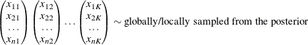
If the length of each chain is less than n, you can augment the the corresponding chain by subsampling the chain itself. Each chain is then sorted with respect to the
nonnormalized posterior density: ![]() . Therefore,
. Therefore,
![\begin{equation*} \begin{pmatrix} x_{11} \\ x_{21} \\ \ldots \\ x_{n1} \end{pmatrix}\begin{pmatrix} x_{12} \\ x_{22} \\ \ldots \\ x_{n2} \end{pmatrix} \ldots \begin{pmatrix} x_{1K} \\ x_{2K} \\ \ldots \\ x_{nK} \end{pmatrix} \rightarrow \begin{pmatrix} x_{[1]1} \\ x_{[2]1} \\ \ldots \\ x_{[n]1} \end{pmatrix}\begin{pmatrix} x_{[1]2} \\ x_{[2]2} \\ \ldots \\ x_{[n]2} \end{pmatrix} \ldots \begin{pmatrix} x_{[1]K} \\ x_{[2]K} \\ \ldots \\ x_{[n]K} \end{pmatrix}\end{equation*}](images/etsug_qlim0357.png)
The final step is to use a multinomial sampler to resample each row i with weights proportional to the nonnormalized posterior densities:
The resulting posterior sample
is a good approximation of the posterior distribution that is characterized by multiple modes.
The MCMC methods can generate samples from the posterior distribution. The correct implementation of these methods often requires the stationarity analysis, the convergence analysis and the accuracy analysis of the posterior samples. These analyses usually imply the following:
-
initialization of the proposal distribution
-
initialization of the chains (starting values)
-
determination of the burn-in
-
determination of the length of the chains.
In more general terms, this determination is equivalent to deciding whether the samples are drawn from the posterior distribution (stationarity analysis), and whether the number of samples is large enough to accurately approximate the posterior distribution (accuracy analysis). You can use the AUTOMCMC option to automate and facilitate the stationary analysis and the accuracy analysis.
The algorithm consists of two phases. In the first phase, the stationarity phase, the algorithm tries to generate stationary samples from the posterior distribution. In the second phase, the accuracy phase, the algorithm searches for an accurate representation of the posterior distribution. The algorithm implements the following tools:
-
Geweke test to check stationarity
-
Heidelberger-Welch test to check stationarity and provide a proxy for the burn-in
-
Heidelberger-Welch half-test to check the accuracy of the posterior mean
-
Raftery-Lewis test to check the accuracy of a given percentile (indirectly proving a proxy for the number of required samples)
-
effective sample size analysis to determine a proxy of the number of required samples
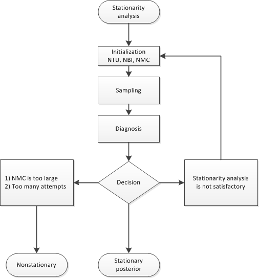
During the stationarity phase, the algorithm searches for stationarity. The number of attempts that the algorithm makes is determined by the option ATTEMPTS=number. During each attempt, a preliminary tuning stage chooses a proposal distribution for the MCMC sampler. At the end of the preliminary tuning phase, the algorithm analyzes tests for the stationarity of the samples. If the percentage of successful stationary tests is equal to or greater than the percentage that is indicated by the option TOL=value, then the posterior sample is considered to be stationary. If the sample cannot be considered stationary, then the algorithm attempts to achieve stationarity by changing some of the initialization parameters as follows:
-
increasing the number of tuning samples (NTU)
-
increasing the number of posterior samples (NMC)
-
increasing the burn-in (NBI)
Figure 22.8 shows a flowchart of the algorithm as it searches for stationarity.
You can initialize NMC=M, NBI=B, and NTU=T during the stationarity phase by specifying NMC, NBI, and NTU as options in the BAYES statement. You can also change the minimum stationarity acceptance ratio of successful stationarity tests that are needed to exit the stationarity phase. By default, TOL=0.95. For example:
   proc qlim data=dataset;
      ...;
      bayes nmc=M nbi=B ntu=T automcmc=( stationarity=(tol=0.95) );
      ...;
   run;
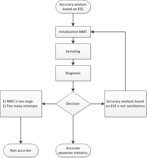
During the accuracy phase, the algorithm attempts to determine how many posterior samples are needed. The number of attempts is determined by the option ATTEMPTS=number. You can choose between two different approaches to study the accuracy:
-
accuracy analysis based on the effective sample size (ESS)
-
accuracy analysis based on the Heidelberger-Welch half-test and the Raftery-Lewis test
If you choose the effective sample size approach, you must provide the minimum number of effective samples that are needed. You can also change the tolerance for the ESS accuracy analysis (by default, TOL=0.95). For example:
   proc qlim data=dataset;
      ...;
      bayes automcmc=(targetess=N accuracy=(tol=0.95));
      ...;
   run;
Figure 22.9 shows a flowchart of the algorithm based on the effective sample size approach to determine whether the samples provide an accurate representation of the posterior distribution.
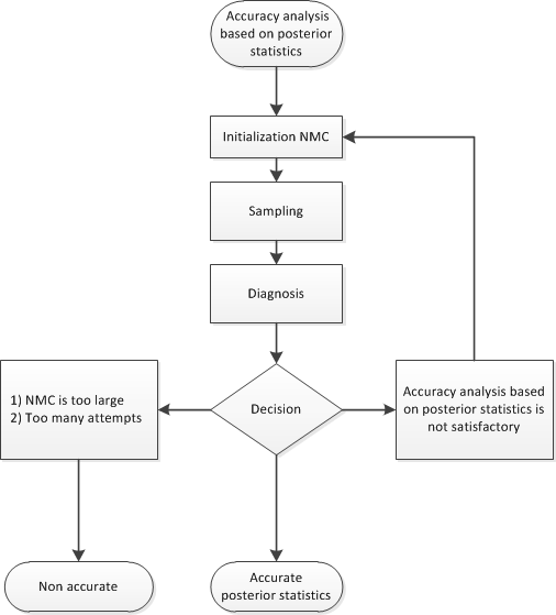
If you choose the accuracy analysis based on the Heidelberger-Welch half-test and the Raftery-Lewis test (the default option), then you might want to choose a posterior quantile of interest for the Raftery-Lewis test (by default, 0.025). You can also change the tolerance for the accuracy analysis (by default, TOL=0.95). Notice that the Raftery-Lewis test produces a proxy of the number of posterior sample required. In each attempt, the current number of posterior samples is compared to this proxy. If the proxy is greater than the current nmc, then the algorithm reinitializes itself. To control this reinitialization, you can use the option RLLIMITS=(LB=lb UB=ub). In particular, there are three cases
-
if the proxy is greater than ub, then NMC is set equal to ub,
-
if the proxy is less than lb, then NMC is set equal to lb,
-
if lb is less than the proxy, which is less than ub, then NMC is set equal to the proxy.
For example:
   proc qlim data=dataset;
      ...;
      bayes raftery(q=0.025) automcmc=( accuracy=(tol=0.95 targetstats=(rllimits=(lb=k1 ub=k2))) );
      ...;
   run;
Figure 22.10 shows a flowchart of the algorithm based on the Heidelberger-Welch half-test and the Raftery-Lewis test approach to determine whether the posterior samples provide an accurate representation of the posterior distribution.
Figure 22.10: Flowchart of the AUTOMCMC Algorithm: Accuracy Analysis Based on the Heidelberger-Welch Half-test and the Raftery-Lewis Test
[13] Roberts and associates demonstrate that the relationship between acceptance probability and scale in a random walk Metropolis
scheme is ![]() , where
, where ![]() is the scale, p is the acceptance rate,
is the scale, p is the acceptance rate, ![]() is the CDF of a standard normal, and
is the CDF of a standard normal, and ![]() ,
, ![]() is the density function of samples (Roberts, Gelman, and Gilks, 1997; Roberts and Rosenthal, 2001). This relationship determines the updating scheme, with
is the density function of samples (Roberts, Gelman, and Gilks, 1997; Roberts and Rosenthal, 2001). This relationship determines the updating scheme, with ![]() replaced by the identity matrix to simplify calculation.
replaced by the identity matrix to simplify calculation.