The PANEL Procedure
- Overview
- Getting Started
-
Syntax

-
DetailsSpecifying the Input DataSpecifying the Regression ModelUnbalanced DataMissing ValuesComputational ResourcesRestricted EstimatesNotationOne-Way Fixed-Effects ModelTwo-Way Fixed-Effects ModelBalanced PanelsUnbalanced PanelsFirst-Differenced Methods for One-Way and Two-Way ModelsBetween EstimatorsPooled EstimatorOne-Way Random-Effects ModelTwo-Way Random-Effects ModelParks Method (Autoregressive Model)Da Silva Method (Variance-Component Moving Average Model)Dynamic Panel EstimatorLinear Hypothesis TestingHeteroscedasticity-Corrected Covariance MatricesHeteroscedasticity- and Autocorrelation-Consistent Covariance MatricesR-SquareSpecification TestsPanel Data Poolability TestPanel Data Cross-Sectional Dependence TestPanel Data Unit Root TestsLagrange Multiplier (LM) Tests for Cross-Sectional and Time EffectsTests for Serial Correlation and Cross-Sectional EffectsTroubleshootingCreating ODS GraphicsOUTPUT OUT= Data SetOUTEST= Data SetOUTTRANS= Data SetPrinted OutputODS Table Names
-
Example
- References
The HCCME= option in the MODEL statement selects the type of heteroscedasticity-consistent covariance matrix. In the presence of heteroscedasticity, the covariance matrix has a complicated structure that can result in inefficiencies in the OLS estimates and biased estimates of the covariance matrix. The variances for cross-sectional and time dummy variables and the covariances with or between the dummy variables are not corrected for heteroscedasticity in the one-way and two-way models. Whether or not HCCME is specified, they are the same. For the two-way models, the variance and the covariances for the intercept are not corrected.[4]
Consider the simple linear model:
This discussion parallels the discussion in Davidson and MacKinnon 1993, pp. 548–562. For panel data models, we apply HCCME on the transformed data(![]() and
and ![]() ). In other words, we first remove the random or fixed effects through transforming/demean the data[5], then correct heteroscedasticity (also auto-correlation with HAC option) in the residual. The assumptions that make the linear
regression best linear unbiased estimator (BLUE) are
). In other words, we first remove the random or fixed effects through transforming/demean the data[5], then correct heteroscedasticity (also auto-correlation with HAC option) in the residual. The assumptions that make the linear
regression best linear unbiased estimator (BLUE) are ![]() and
and ![]() , where
, where ![]() has the simple structure
has the simple structure ![]() . Heteroscedasticity results in a general covariance structure, so that it is not possible to simplify
. Heteroscedasticity results in a general covariance structure, so that it is not possible to simplify ![]() . The result is the following:
. The result is the following:
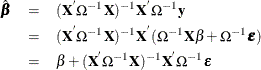
As long as the following is true, then you are assured that the OLS estimate is consistent and unbiased:
If the regressors are nonrandom, then it is possible to write the variance of the estimated ![]() as the following:
as the following:
The effect of structure in the covariance matrix can be ameliorated by using generalized least squares (GLS), provided that
![]() can be calculated. Using
can be calculated. Using ![]() , you premultiply both sides of the regression equation,
, you premultiply both sides of the regression equation,
where ![]() denotes the Cholesky root of
denotes the Cholesky root of ![]() . (that is,
. (that is, ![]() with
with ![]() lower triangular).
lower triangular).
The resulting GLS ![]() is
is
Using the GLS ![]() , you can write
, you can write
The resulting variance expression for the GLS estimator is
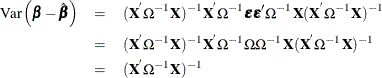
The difference in variance between the OLS estimator and the GLS estimator can be written as
By the Gauss-Markov theorem, the difference matrix must be positive definite under most circumstances (zero if OLS and GLS
are the same, when the usual classical regression assumptions are met). Thus, OLS is not efficient under a general error structure.
It is crucial to realize that OLS does not produce biased results. It would suffice if you had a method for estimating a consistent
covariance matrix and you used the OLS ![]() . Estimation of the
. Estimation of the ![]() matrix is certainly not simple. The matrix is square and has
matrix is certainly not simple. The matrix is square and has ![]() elements; unless some sort of structure is assumed, it becomes an impossible problem to solve. However, the heteroscedasticity
can have quite a general structure. White (1980) shows that it is not necessary to have a consistent estimate of
elements; unless some sort of structure is assumed, it becomes an impossible problem to solve. However, the heteroscedasticity
can have quite a general structure. White (1980) shows that it is not necessary to have a consistent estimate of ![]() . On the contrary, it suffices to calculate an estimate of the middle expression. That is, you need an estimate of:
. On the contrary, it suffices to calculate an estimate of the middle expression. That is, you need an estimate of:
This matrix, ![]() , is easier to estimate because its dimension is K. PROC PANEL provides the following classical HCCME estimators for
, is easier to estimate because its dimension is K. PROC PANEL provides the following classical HCCME estimators for ![]() :
:
The matrix is approximated by:
-
HCCME=N0:
![\[ \sigma ^2 \mb{X} ^{'}\mb{X} \]](images/etsug_panel0607.png)
This is the simple OLS estimator. If you do not specify the HCCME= option, PROC PANEL defaults to this estimator.
-
HCCME=0:
![\[ \sum _{i = 1} ^{N} \sum _{t=1}^{T_ i} \hat{\epsilon }_{it} ^{2}\mb{x} _{it} \mb{x} _{it} ^{'} \]](images/etsug_panel0608.png)
where N is the number of cross sections and
 is the number of observations in ith cross section. The
  is from the tth observation in the ith cross section, constituting the
  th row of the matrix
  . If the CLUSTER option is specified, one extra term is added to the preceding equation so that the estimator of matrix
  is
is
![\[ \sum _{i = 1} ^{N} \sum _{t=1}^{T_ i} \hat{\epsilon }_{it} ^{2}\mb{x} _{it} \mb{x} _{it} ^{'} +\sum _{i = 1} ^{N} \sum _{t=1}^{T_ i} \sum _{s=1}^{t-1} \hat{\epsilon }_{it}\hat{\epsilon }_{is} \left(\mb{x} _{it} \mb{x} _{is} ^{'}+\mb{x} _{is} \mb{x} _{it} ^{'}\right) \]](images/etsug_panel0613.png)
The formula is the same as the robust variance matrix estimator in Wooldridge (2002, p. 152) and it is derived under the assumptions of section 7.3.2 of Wooldridge (2002).
-
HCCME=1:
![\[ \frac{M}{M-K}\sum _{i = 1} ^{N} \sum _{t=1}^{T_ i} \hat{\epsilon }_{it} ^{2}\mb{x} _{it} \mb{x} _{it} ^{'} \]](images/etsug_panel0614.png)
where M is the total number of observations,
 , and K is the number of parameters. With the CLUSTER option, the estimator becomes
![\[ \frac{M}{M-K}\sum _{i = 1} ^{N} \sum _{t=1}^{T_ i} \hat{\epsilon }_{it} ^{2}\mb{x} _{it} \mb{x} _{it} ^{'} +\frac{M}{M-K}\sum _{i = 1} ^{N} \sum _{t=1}^{T_ i} \sum _{s=1}^{t-1} \hat{\epsilon }_{it}\hat{\epsilon }_{is} \left(\mb{x} _{it} \mb{x} _{is} ^{'} + \mb{x} _{is} \mb{x} _{it} ^{'}\right) \]](images/etsug_panel0616.png)
The formula is similar to the robust variance matrix estimator in Wooldridge (2002, p. 152) with the heteroskedasticity adjustment term
 .
.
-
HCCME=2:
![\[ \sum _{i = 1} ^{N} \sum _{t=1}^{T_ i} \frac{\hat{\epsilon }_{it} ^{2}}{1 - \hat{h}_{it}}\mb{x} _{it} \mb{x} _{it} ^{'} \]](images/etsug_panel0618.png)
The
 term is the th diagonal element of the hat matrix. The expression for is
  . The hat matrix attempts to adjust the estimates for the presence of influence or leverage points. With the CLUSTER option,
the estimator becomes
. The hat matrix attempts to adjust the estimates for the presence of influence or leverage points. With the CLUSTER option,
the estimator becomes
![\[ \sum _{i = 1} ^{N} \sum _{t=1}^{T_ i} \frac{\hat{\epsilon }_{it} ^{2}}{1 - \hat{h}_{it}}\mb{x} _{it} \mb{x} _{it} ^{'} +2\sum _{i = 1} ^{N} \sum _{t=1}^{T_ i} \sum _{s=1}^{t-1} \frac{\hat{\epsilon }_{it}}{\sqrt {1 - \hat{h}_{it}}}\frac{\hat{\epsilon }_{is}}{\sqrt {1 - \hat{h}_{is}}} \left(\mb{x} _{it} \mb{x} _{is} ^{'} + \mb{x} _{is} \mb{x} _{it} ^{'}\right) \]](images/etsug_panel0621.png)
The formula is similar to the robust variance matrix estimator in Wooldridge (2002, p. 152) with the heteroskedasticity adjustment.
-
HCCME=3:
![\[ \sum _{i = 1} ^{N} \sum _{t=1}^{T_ i} \frac{\hat{\epsilon }_{it} ^{2}}{(1 - \hat{h}_{it})^2}\mb{x} _{it} \mb{x} _{it} ^{'} \]](images/etsug_panel0622.png)
With the CLUSTER option, the estimator becomes
![\[ \sum _{i = 1} ^{N} \sum _{t=1}^{T_ i} \frac{\hat{\epsilon }_{it} ^{2}}{(1 - \hat{h}_{it})^2}\mb{x} _{it} \mb{x} _{it} ^{'} +2\sum _{i = 1} ^{N} \sum _{t=1}^{T_ i} \sum _{s=1}^{t-1} \frac{\hat{\epsilon }_{it}}{1 - \hat{h}_{it}}\frac{\hat{\epsilon }_{is}}{1 - \hat{h}_{is}} \left(\mb{x} _{it} \mb{x} _{is} ^{'} + \mb{x} _{is} \mb{x} _{it} ^{'}\right) \]](images/etsug_panel0623.png)
The formula is similar to the robust variance matrix estimator in Wooldridge (2002, p. 152) with the heteroskedasticity adjustment.
-
HCCME=4: PROC PANEL includes this option for the calculation of the Arellano (1987) version of the White (1980) HCCME in the panel setting. Arellano’s insight is that there are
 covariance matrices in a panel, and each matrix corresponds to a cross section. Forming the White HCCME for each panel, you
need to take only the average of those estimators that yield Arellano. The details of the estimation follow. First, you arrange the data such that the first cross
section occupies the first
covariance matrices in a panel, and each matrix corresponds to a cross section. Forming the White HCCME for each panel, you
need to take only the average of those estimators that yield Arellano. The details of the estimation follow. First, you arrange the data such that the first cross
section occupies the first  observations. You treat the panels as separate regressions with the form:
![\[ \mb{y} _\mi {i} = \alpha _\mi {i} \mb{i} + \mb{X} _\mi {is} \tilde{\bbeta } + \bepsilon _\mi {i} \]](images/etsug_panel0626.png)
The parameter estimates
 and
and  are the result of least squares dummy variables (LSDV) or within estimator regressions, and
  is a vector of ones of length . The estimate of the ith cross section’s
  matrix (where the
  subscript indicates that no constant column has been suppressed to avoid confusion) is
  . The estimate for the whole sample is:
![\[ \mb{X} _\mi {s} ^{'}\Omega \mb{X} _\mi {s} = \sum _\mi {i = 1} ^{N}\mb{X} _\mi {i} ^{'}\Omega \mb{X} _\mi {i} \]](images/etsug_panel0633.png)
The Arellano standard error is in fact a White-Newey-West estimator with constant and equal weight on each component. In the between estimators, selecting HCCME=4 returns the HCCME=0 result since there is no 'other' variable to group by.
In their discussion, Davidson and MacKinnon (1993, p. 554) argue that HCCME=1 should always be preferred to HCCME=0. Although HCCME=3 is generally preferred to 2 and 2 is preferred to 1, the calculation of HCCME=1 is as simple as the calculation of HCCME=0. Therefore, it is clear that HCCME=1 is preferred when the calculation of the hat matrix is too tedious.
All HCCME estimators have well-defined asymptotic properties. The small sample properties are not well-known, and care must exercised when sample sizes are small.
The HCCME estimator of ![]() is used to drive the covariance matrices for the fixed effects and the LaGrange multiplier standard errors. Robust estimates
of the covariance matrix for
is used to drive the covariance matrices for the fixed effects and the LaGrange multiplier standard errors. Robust estimates
of the covariance matrix for ![]() imply robust covariance matrices for all other parameters.
imply robust covariance matrices for all other parameters.
[4] The dummy variables are removed by the within transformations, so their variances and covariances cannot be calculated the same way as the other regressors. They are recovered by the formulas listed in the sections One-Way Fixed-Effects Model and Two-Way Fixed-Effects Model. The formulas assume homoscedasticity, so they do not apply when HCCME is specified. Therefore, standard errors, variances, and covariances are reported only when the HCCME option is ignored. HCCME standard errors for dummy variables and intercept can be calculated by the dummy variable approach with the pooled model.
[5] Please refer to One-Way Fixed-Effects Model, Two-Way Fixed-Effects Model, One-Way Random-Effects Model, and Two-Way Random-Effects Model for details about transforming the data.